 Eli Bendersky's website
 The Fourier series is a great tool for analyzing periodic functions. But what about functions that don’t repeat? We’ve seen that we can compute Fourier series for a non-periodic function defined on a finite interval, as long as we don’t care about its behavior beyond that interval.
Let’s extend this idea to functions that never repeat; that is, non-periodic functions defined on the interval .
Visualizing Fourier series for non-repeating functions
To motivate the subject ahead, let’s look back at the example used in the earlier post about Fourier series:
With an odd extension into . In that post, to make the Fourier series work, we assumed keeps repeating with a period on the entire axis. Here, let’s face the reality that it does not - in fact - repeat, and observe how our Fourier series work out.
Recall that the Fourier series approximating are the sine series (since it’s an odd function):
The following visualization is interactive. By default, it shows (with its odd extension) and no Fourier series approximation. We’ll proceed by a series of steps and observe the outcome:
Step 1: set to some non-zero number; already at 3, the approximation is very good.
The frequency spacing is (this is the coefficient of in the sines). Note that the Fourier series repeats every , as expected.
Step 2: increase to 6. This means our series are constructed assuming has a period of 12, not 4. Note how the Fourier series look now - they repeat every 12, and they don’t match as well as before. We can increase to a higher number to make the match better. As grows, the spacing between adjacent frequencies decreases.
Step 3: increase to 10. We no longer see the repetitions, so feel free to increase the values of x min and x max until you do. Note again that we need to add more and more coefficients to match better with this larger , and the spacing adjacent frequencies grows smaller.
Increasing means our function repeats at larger and larger intervals. The logical conclusion of this progression is to ask - what happens if the function never repeats, meaning ? While not mathematically rigorous, the visual experiment here lets us make some conjectures: we’ll likely need an infinite number of coefficients for a good approximation, and moreover, the spacing between these coefficients will tend to zero.
In other words, instead of a discrete set of coefficients, we’ll end up with a continuous line, or function. The function produced by this process is the Fourier transform of , and the next section shows its mathematical derivation.
Fourier series with leading to Fourier transform
In these notes, we’ll be using the complex exponential formulation of Fourier series:
With:
We’re interested in a non-periodic defined on the interval . So we’ll be exploring the above equations for .
First, let’s make a slight change of notation. Instead of writing formulae in terms of the period (), we’ll be using the n-th harmonic angular frequency :
So we can slightly rewrite our series as:
Using as the difference between two consecutive frequencies:
Using this notation, is expressed as:
So far there are no new insights here, just some new notation. Now we’re going to use it to facilitate the next step.
Since , then . Let’s calculate the limit of the Fourier series representation of when :
And substitute the latest into this equation, changing its dummy integration variable from to to avoid confusion [1]
Reordering slightly, and also replacing by in the complex exponents:
Looking at the limit with the sum carefully, this is a Riemann sum (see Appendix A)! is the "sampled" version of , and . We can therefore replace it by an integral, changing to and to [2]:
The inner integral is called the Fourier transform of and denoted [3]:
And the full equation for is then the inverse Fourier transform:
Example calculation of Fourier transform
Let’s take our favorite odd triangular pulse example and calculate its Fourier transform. The function’s mathematical definition and plot are shown earlier in this post. Note that we’re not extending this function periodically - it’s zero beyond the range ; this is exactly why we need the Fourier transform here - as we’ve seen, Fourier series won’t do because the function they reconstruct eventually starts repeating.
We’re looking to find:
To calculate the integral, let’s decompose the complex exponent using Euler’s formula:
Since our is odd, the first integral is zero. Also is even, so we can write:
We’ve already calculated a very similar integral in the post on Fourier series, so let’s just skip to the result:
The only remaining difficulty is its value at 0, which seems undefined at first (division by zero). However, note that as , the numerator also tends to 0, so we can use L’Hopital’s rule (twice!) to find that:
Therefore:
This function is complex-valued; in fact, it’s purely imaginary. How do we visualize it? A common way to visualize complex-valued functions is by plotting their magnitude and phase separately.
The magnitude of is:
Since is purely imaginary, there are only two options for the phase:
When the numerator is positive, we get a negative imaginary number with phase , and when the numerator is negative, we get a positive imaginary number with phase . Finally, when (which happens at , by our earlier analysis, but also whenever is a whole multiple of ), the phase is undefined.
Here’s the magnitude and phase of plotted against :
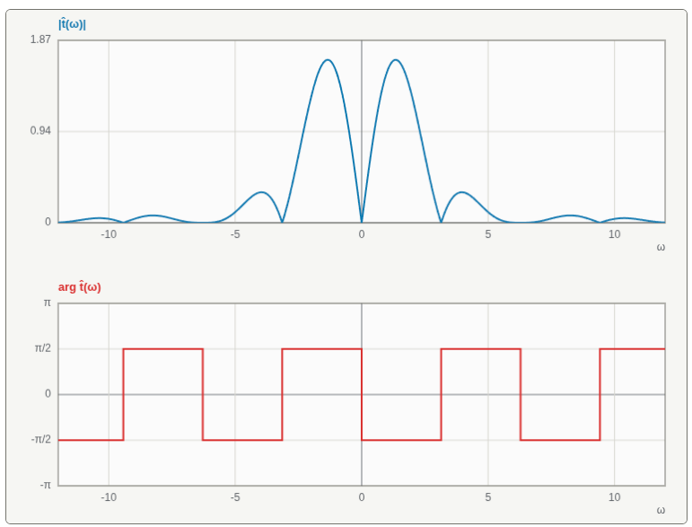
It is common to talk about as the frequency domain representation of .
The frequency domain representation of functions
When the functions we’re working with have time as their domain (e.g. the in represents time), which is often the case in the study of signals and systems, the Fourier transform can be seen as computing the frequency domain representation of the function.
Here’s the Fourier transform formula again:
It takes - the time domain representation of a function, and converts it to - a frequency domain representation. For well-behaved functions, these two representations are dual - each one describes the function completely, just in a different way.
To convert back from a frequency domain representation to the time domain, we use the inverse Fourier transform:
While a time-domain plot () shows how a signal changes over time, a frequency-domain plot () shows how the signal is distributed across all possible frequencies. Moreover, as we’ve seen, is complex valued. Each frequency therefore has both a magnitude and a phase: the magnitude tells us how strongly that frequency contributes, while the phase tells us how that component is shifted.
The frequency domain is extremely useful in signal analysis; for example, when designing filters.
The Fourier transform also has a number of properties that are very useful in signal analysis and processing. But first, let’s discuss what a "well-behaved function" means for the purpose of applying Fourier transforms.
Existence condition for the Fourier transform
The simplest existence condition for Fourier transforms is absolute integrability (also known as Lebesgue integrable):
With this condition, exists on the entire domain, is continuous and vanishes (tends to 0) as [4].
While this condition is sufficient, it’s not necessary; there are less well-behaved functions that also have Fourier transforms defined with some limitations. In these notes, we’re mostly interested in well-behaved functions that are used in real-world engineering, so we won’t discuss the other cases.
Another assumption commonly made for real-world functions is that they vanish (tend to 0) as . While this is not a direct outcome of absolute integrability [5], it’s a reasonable assumption in engineering. After all, real-world signals have finite energies.
Intuitively, when we also assume is uniformly continuous, the assumption of vanishing at is a logical conclusion, because otherwise how can the total area for be finite?
An important outcome of this discussion is that the Fourier transform is unsuitable for periodic functions. Functions that repeat at intervals are not absolute integrable. For periodic functions, we use Fourier series.
Some useful properties of Fourier transforms
Linearity
The Fourier transform is a linear operator, because the integral is linear:
So is the inverse Fourier transform; it’s similarly easy to show that:
Scaling
If we scale the domain of a function by a constant, its transform changes only slightly:
Let’s do the variable substitution :
This is the Fourier transform evaluated at , so:
There’s one small caveat here; when is negative, the integral bounds should be flipped, causing a minus sign in front of the transform. So we can write:
Which works for any .
This property is intuitive when thinking about signals: suppose , then means the signal is compressed in the time domain by a factor . The scaling property says that the frequency domain is expanded using the same factor; in other words, the higher frequencies become more prominent because we need sharper transitions to represent the compressed signal.
Time shifting
What happens to the Fourier transform if we time-shift the input signal by some constant: . By definition:
Substituting , we get , so:
Transform of a derivative
An extremely useful property that’s often employed in the solution of partial differential equations; let’s calculate the Fourier transform of the derivative of :
We’ll use integration by parts, where and . Therefore, and :
Recall the assumption made in the "Existence condition..." section about vanishing at infinities. So the first part of the equation above is zero, and we’re left with:
Transform of convolution
The convolution between two continuous functions and is defined as:
Let’s calculate the Fourier transform of this function:
This step of combining the integrals into a double integral, as well as the next step (changing the order of integration) is possible due to Fubini’s theorem and our assumption that and are Lebesgue integrable.
Switch order of integration:
Now, in the inner integral doesn’t depend on , so we can pull it out:
The inner integral is just the Fourier transform of a time-shifted , so we can write:
And the remaining integral is the Fourier transform of , so:
Convolution in the time domain translates to multiplication in the frequency domain! This result is so important in signal processing that it’s called the convolution theorem.
Appendix A: Riemann sum and the definite integral
Suppose we have some function and we want to know the area bounded between this function’s graph and the axis in a certain interval . One way to do this is to take a partition of the interval:
And calculate the area under for every element of the partition. We can then approximate such sub-areas by rectangles, as follows:
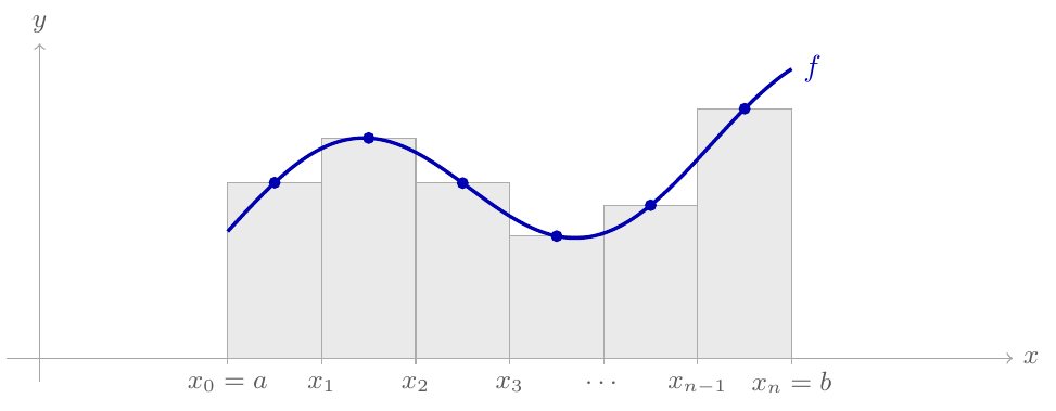
We’ll denote the area of each rectangle as :
- is the width of one interval (assuming a uniform partition, but the math works just as well for non-uniform ones).
- is some value in the interval .
There are many ways to choose which point of the interval to denote as : left point (), right point (), mid-point between the two (which is what our plot shows) or anything in between. The distinction doesn’t really matter for our purpose, as we will soon see.
We can approximate the area under the curve of in the interval with the Riemann sum, using a uniform partition:
If is continuous on , then as :
This is known as the Riemann integral, or just the definite integral. The limit is why the exact choice of doesn’t matter: as we have , and all points within are equally good.
| [1] | Note that is not a function of ; in its definition, only serves as a dummy integration variable and can be called anything we choose. When we substitute into the equation for , which is a function of , we have to be careful. Thus the renaming. |
| [2] | Note we apply the limit; therefore, the bounds of the inner integral (in the square brackets) are now also between and |
| [3] | We change the dummy integration variable back to here, for consistency. Once again, since is just the integration variable and the integral is definite, the final result doesn’t depend on . It’s a function of . |
| [4] | The vanishing at infinity part is the Riemann-Lebesgue lemma; you can find a proof on Wikipedia |
| [5] | A pathological absolute-integrable function can have spikes at infinity but still have a finite total area. |