 Eli Bendersky's website
In the previous post on this topic, we’ve seen how the Discrete-Time Fourier Series (DTFS) and transform (DTFT) are used to analyze infinite-duration periodic and non-periodic discrete signals. Now, it’s time to turn to realistic digital signal processing where signals are not only discrete, but also finite in duration.
Analyzing signal samples
Suppose we have samples of a signal - it’s a list of numbers:
We want to analyze the frequencies present in this signal; in other words, to find the coefficients in a series of complex exponentials that reconstructs the signal. One option is to assume that is an infinite domain signal with zero values outside our samples, and then compute its DTFT:
However, this is a continuous function of frequency , so it’s difficult compute on an actual computer; we cannot evaluate and store it for all , so we have to choose which to compute it for. We'll soon see how this choice is made.
The Discrete Fourier Transform (DFT)
But there's an alternative way to look at the problem. We only have samples of the signal , so we can assume they represent a single period of a periodic signal. And in that case, we can use DTFS; recall that the coefficients of the series are:
As we’ve seen in the post on the DTFS, this series can be used to reconstruct a discrete, periodic signal precisely. Since our signal is finite and we assume it’s just one period of a periodic signal, it means we can also reconstruct precisely using a DTFS.
This is the main insight behind the Discrete Fourier Transform (DFT). First, by convention [1] we define:
And then:
This is called the Discrete Fourier Transform of . The term transform may be a bit puzzling here - after all, we’re just using the series coefficients - so isn’t it more proper to just say series? Perhaps, though in mathematics a transform has a pretty general meaning of "a mapping that takes a mathematical object and produces another object"; in that sense, "transform" is proper here because we take an object - and produce another object - .
Moreover, DFT and DTFT are intimately related. Recall how we said earlier that the DTFT is tricky to compute because is a continuous variable? Well, the DFT gives us a way to sample that variable into the discrete domain:
So the DFT can be seen as exactly equally spaced samples of the DTFT.
Computing the DFT
Since the goal of this post is specifically to demonstrate computable methods of applying Fourier analysis to discrete digital signals, here’s the Python code to calculate the DFT of a signal:
def dft(x):
    """Return X[k] = sum_n x[n] exp(-2 pi i k n / N)."""
    N = len(x)
    n = np.arange(N)
    X = np.empty(N, dtype=complex)
    for k in range(N):
        weights = np.exp(-2j * np.pi * k * n / N)
        X[k] = np.sum(x * weights)
    return X
It shouldn’t be hard to see the correspondence between this code and the mathematical formula for . Python’s Numpy code is vectorized by default, so the weights array is computed in whole for every k (because n is an array of indices ).
DFT and the complex roots of unity
In my earlier post on the complex roots of unity, we’ve seen how powers of the roots of unity form an orthogonal basis for . Now let’s show the beautiful theoretical connection between this fact and the DFT.
Recall that the -th roots of unity can be written as:
Since all are just powers of , we can write them as:
The conjugates of the roots of unity are roots of unity themselves:
With being the same as , so when we enumerate all the roots of unity, we’re also enumerating their conjugates, just in a reversed order.
With that in mind, let’s denote [2] , and examine the sequence:
The vectors formed by (element-wise) raising to integer powers from to can be collected into a matrix:
In the roots of unity post, we’ve proven that the rows of this matrix form an orthogonal basis over . In other words, any vector in can be represented as a linear combination of the rows of .
I hope you can see where this is going! Let’s consider the signal as a column vector in . The DFT of can be computed by multiplying by the matrix :
Take a minute to convince yourself this is true, by working through the multiplication for a specific row , e.g. is computed via row-column multiplication the third row (counting from 0) of and .
Our is called the Fourier Matrix or the DFT Matrix. Previously we’ve seen Python code that directly computes the DFT; here’s a version that does this via the matrix multiplication approach:
def dft_matrix(N):
    """Construct F[k, n] = W_N**(k*n), where W_N = exp(-2 pi i / N)."""
    # W_N is a primitive N-th root of unity: W_N**N = 1.
    # Its powers give all N roots of z**N - 1 = 0.
    root = np.exp(-2j * np.pi / N)
    indices = np.arange(N)
    # Rows correspond to frequency bins k; columns to sample indices n.
    exponents = np.outer(indices, indices)
    return root**exponents

def dft_via_matrix(x):
    """Compute the DFT as F @ x with the Fourier matrix"""
    return dft_matrix(len(x)) @ x
More than the computational convenience though, there’s theoretical elegance here. Back when we were discussing the continuous Fourier series, we’ve seen how the trigonometric functions (or - equivalently - complex exponentials) form an orthogonal basis for square integrable functions.
Here, we see a similar linear algebra connection in discrete time - the vectors formed from powers of complex roots of unity form an orthogonal basis in and can thus be used to represent any sequence of complex values.
Which brings us to the next topic: reconstructing a signal from its DFT representation.
Inverse DFT: reconstructing the signal
There are two equivalent approaches to find the inverse DFT - the formula we can use to reconstruct given . The first approach is going back to DTFS, where the reconstruction formula is:
Recall that our convention is . Therefore:
This is the Inverse Discrete Fourier Transform formula.
Let’s examine the other approach now, because it uses our linear algebra interpretation in an enlightening way.
Recall the Fourier matrix , and consider - the same matrix where every element is the conjugate of the corresponding element of . If:
Then:
What happens if we multiply by ?
We have seen in the roots of unity post that this amounts to:
In other words:
Where is the identity matrix. Since is a square matrix, any matrix that multiplies with it to give the identity is its inverse:
Recall that in vector form:
Therefore:
With our definition of :
And in sum form:
Which is the same reconstruction formula we obtained from the DTFS. In mathematics, it’s always a good sign when we obtain the same result using different methods!
The linear algebra interpretation here is clear: the vectors formed by the powers of roots of unity form an orthogonal basis over . Therefore, every vector can be represented as a linear combination of these vectors. Moreover, this transformation is invertible, and the original vector can be reconstructed by left-multiplying its DFT vector by .
Example
It’s time for a fully worked example; the entire Python code for this example is available on GitHub; read through its main function, which is well commented.
Recall the sampled triangular signal we’ve used in the previous post; here, let’s use a single cycle:
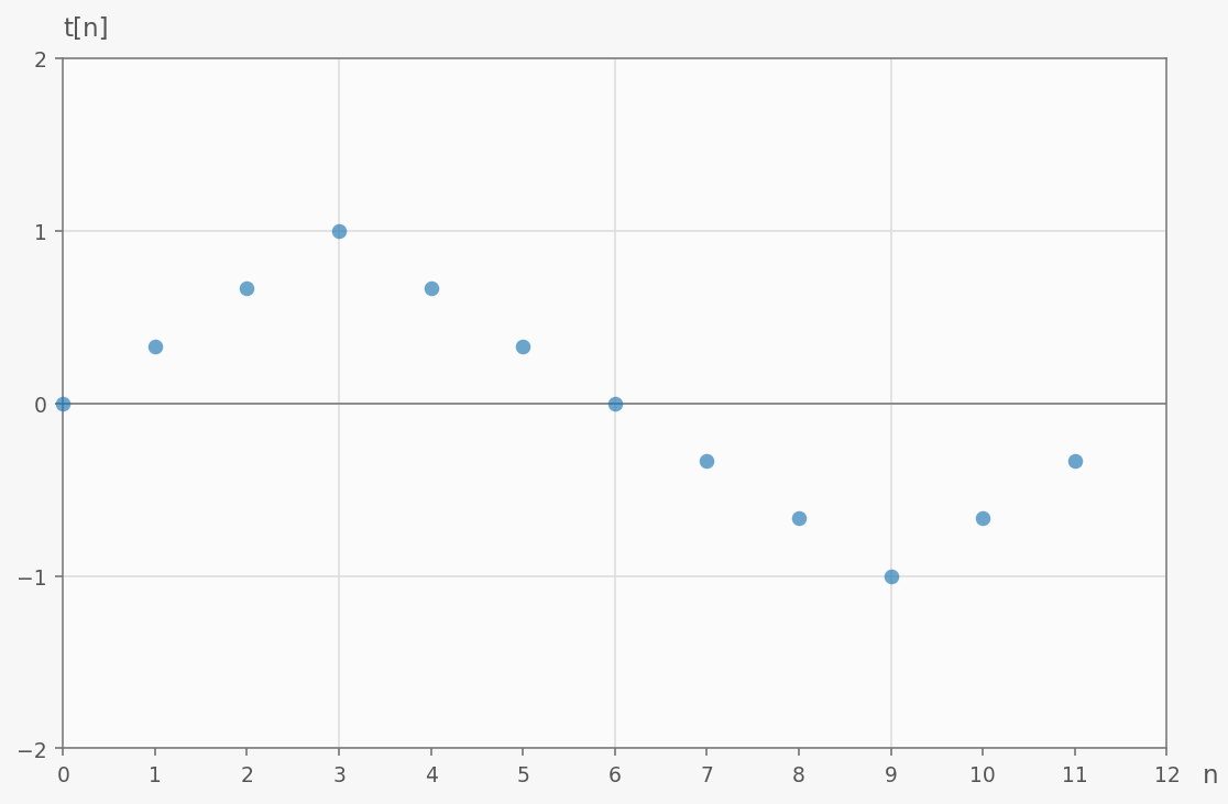
In code, this is just an array of numbers:
x = np.array([0, 1, 2, 3, 2, 1, 0, -1, -2, -3, -2, -1]) / 3
Calculating the DFT of this signal using the code shown earlier produces the following values; remember that consists of complex numbers, so we represent them as a magnitude-phase pair. Phase is only shown for nonzero coefficients, because the phase of zero is undefined [3]:
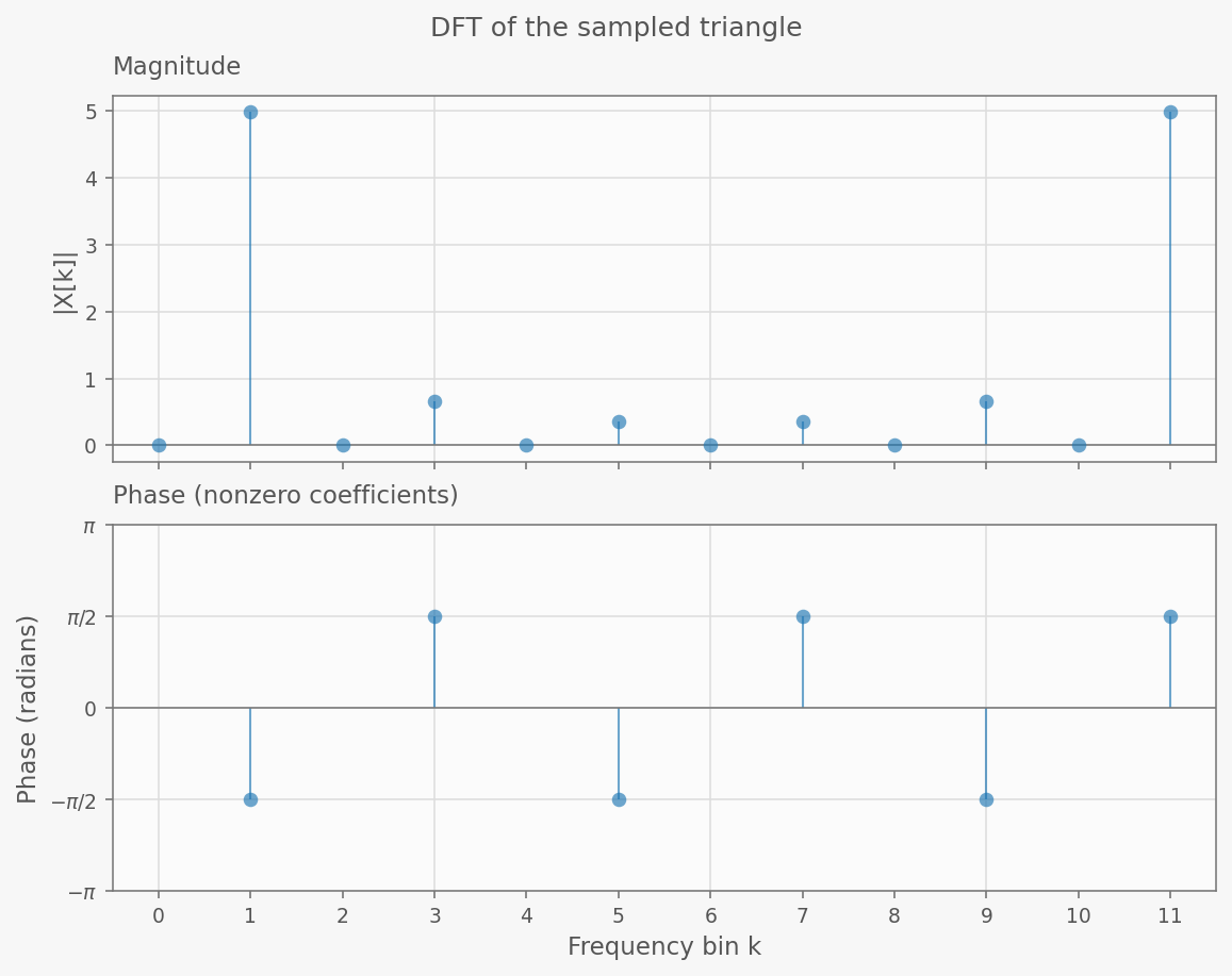
Obviously, we’d get exactly the same numbers by using the matrix multiplication method of computing the DFT. And to reconstruct the signal, we multiply by the computed IDFT matrix to get the original signal back. The reconstruction matches the original signal precisely, with any differences being attributable to floating point round-off.
Efficiently computing the DFT
The sample code contains another method of computing the DFT of this signal - by calling NumPy’s fft.fft function. This refers to the Fast Fourier Transform, which is considered to be one of the most important algorithms of the 20th century. By exploiting the structure of the Fourier matrix , FFT computes the product in operations, compared with for direct matrix-vector multiplication. I plan to cover how this works in a future post.
Appendix: spectral leakage
Looking carefully at the signal used in the Example section above, we see that it’s actually one full cycle out of a sampled triangle wave. This is convenient, because repeating the block reproduces the original triangle wave. But what happens when the samples cover only part of the cycle?
Take for example just the first 10 samples of the triangle wave:
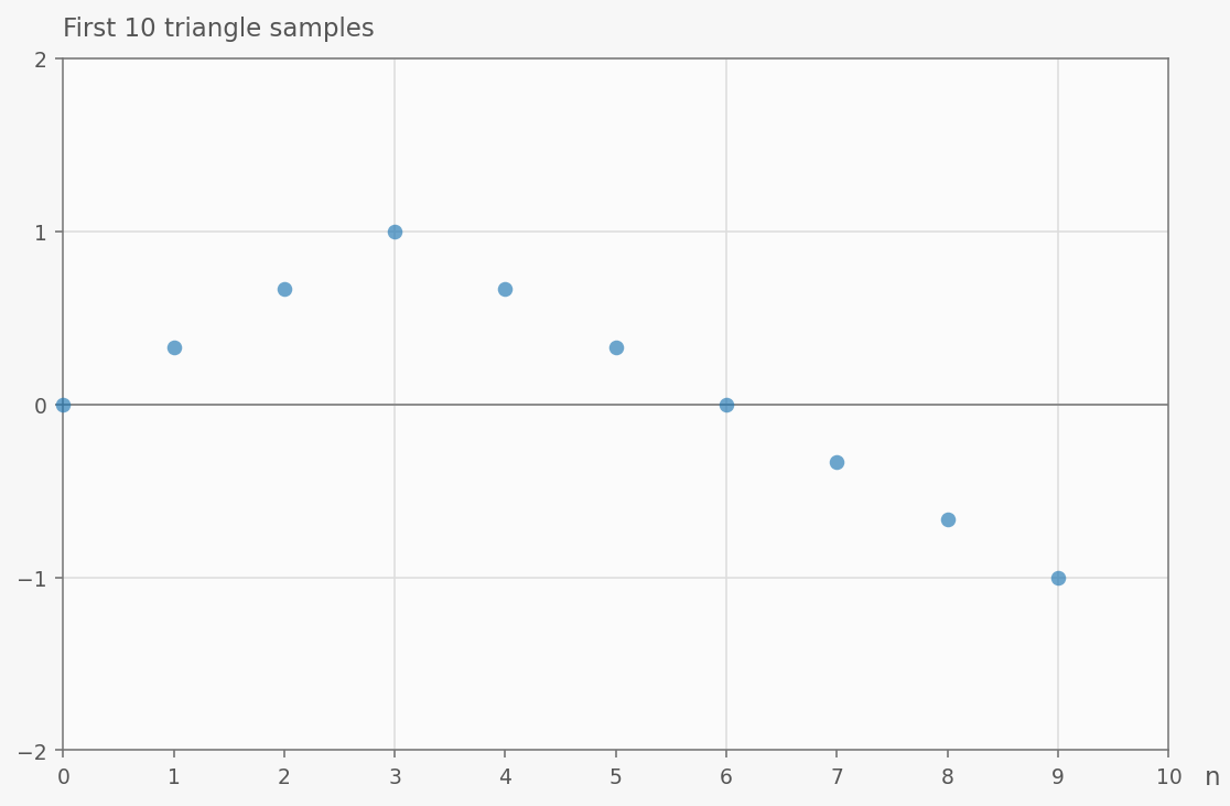
If we naively extend this signal periodically, things won’t line up (there will be a jump at the end of every cycle). We can still calculate its DFT, of course; these are the coefficients we’ll get:
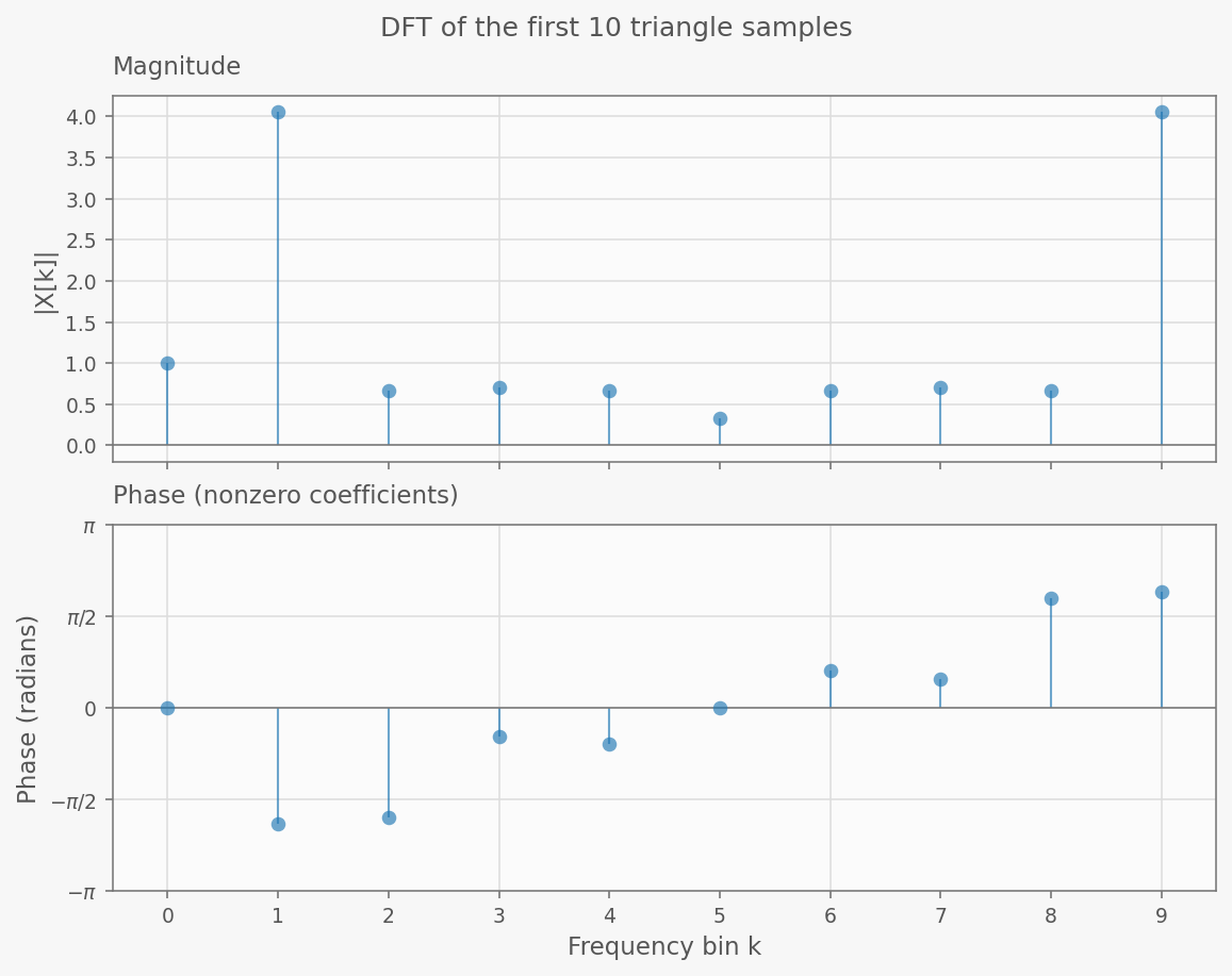
While the coefficients still come in conjugate pairs (because the samples are real), the original triangle’s frequencies no longer coincide with the DFT’s frequency bins, so their contributions spread across multiple bins. This is called spectral leakage.
By applying the IDFT we can still reconstruct the original 10-sample signal perfectly! So if all we need is reconstruction, spectral leakage isn’t an issue; but if we’re doing frequency analysis, it skews the situation somewhat, adding frequencies that didn’t really exist in the underlying triangle wave - just to account for the discontinuity. In real-world signal processing, such issues are usually addressed by applying special window functions to the signal after sampling - these help alleviate leakage by tapering the signal close to zero at the edges.
| [1] | We use the common convention, also used by Numpy by default, with no normalization factor in the forward transform and a factor in the inverse transform. |
| [2] | This is the Greek omega symbol , not the English . The two look very similar - which is alright for our use case - it helps emphasize that using either the roots of unity themselves or their conjugates is completely equivalent here. |
| [3] | Note the symmetry around bin 6; this is expected, because bin 6 represents the root of unity mapping to -1, and all the values following it are equivalent to negative frequencies ( being equivalent to ). Our signal is real, so the magnitudes of negative frequencies will match their positive counterparts, while phase is opposite. |