 Eli Bendersky's website
 Monte Carlo simulations (or methods) is the technique of applying randomness and the Law of large numbers to the solution of various scientific and engineering problems. One of its first documented uses was by Stanislaw Ulam and John von Neumann for nuclear weapon simulations after WWII [1].
In this post I want to provide examples of some simple uses of Monte Carlo simulations. We'll start with the classical example of calculating the value of by throwing darts.
Estimating pi
Suppose we take a square board and inscribe a quarter of a circle into it. We then proceed to throw darts at the board and record whether each dart hits inside or outside the quarter circle. Having thrown many such darts, we calculate the ratio of the darts inside the circle to the total number thrown.
Assuming our darts are distributed uniformly over the square, by the Law of large numbers this ratio should approach the ratio of areas of the quarter circle to the full square .
With a square side length of 1, we have:
Therefore:
Here's a visualization:
π ≈ —
Change the number of samples (dart throws) and click "Run" to regenerate. The code is very simple - here's a slightly sanitized version:
const total = Number(samples.value);
let inside = 0;
for (let i = 0; i < total; i++) {
  const x = Math.random();
  const y = Math.random();
  const inCircle = x * x + y * y <= 1;
  if (inCircle) inside++;
}
estimateValue = 4 * inside / total;
You'll notice that the estimate is relatively poor - even with 1000 samples - if you click "Run" several times, some numbers will be way off mark. While this method does estimate , it's not a particularly good estimate. I find that running ~10 billion samples is necessary to estimate it to 4 digits after the decimal with reasonable reliability.
In general, for independent trials like these, the typical sampling error decreases in proportion to , where N is the number of trials. This means that halving the error requires four times as many samples.
While the estimation may seem whimsical, it's an example of an important class of problems to which Monte Carlo simulation is applied: numerical integration. Our simulation estimates the area under the quarter-circle curve, which is a definite integral.
Many integrals are very difficult to solve analytically, and much research has been done in the area of numerical analysis to develop methods to calculate integrals. Monte Carlo methods are particularly useful for high-dimensional integrals, where other numerical methods can become prohibitively expensive.
Combinatorial simulation - the game of SET
A common use of Monte Carlo methods is estimating complex combinatorial calculations. These often don't have analytical solutions, and enumerating all options is intractable due to the scale of the numbers involved. As an example, let's consider the game of SET. Each SET card has four attributes:
- Number of shapes (1, 2 or 3)
- Color (Red, Green or Purple)
- Shape type (Oval, Diamond or Squiggle)
- Shading (Empty, Striped or Solid)
And the goal is to find a "set" - three cards that are either all different or all the same for each attribute separately. As an example, here's a hand with a single set; see if you can find it [2]:
And the next hand doesn't have any sets:
Here's a question: given a freshly shuffled SET deck, what are the odds that the first 12 cards drawn will have no sets among them? This question is difficult to answer without using a computer.
It's easy to calculate the number of ways to deal a 12-card hand from a deck of 81:
But how many of these hands have no sets? Enumerating 70 trillion SET hands and checking each one can take quite a while, and there is no straightforward counting formula to answer this question. Some clever methods can be employed to leverage symmetries and other mathematical properties of SET to cut down this search space considerably. Donald Knuth himself worked on this problem and came up with a neat program (setset-all on his programs page) that found 2,284,535,476,080 such hands. Therefore, the answer to our question is:
There's a 3.23% chance that a randomly drawn hand of 12 cards from a full deck of SET will have no set in it.
Let's see how we can use a Monte Carlo simulation to answer this question with relatively small effort, without deep knowledge of the mathematical properties of SET that enable cutting down the search space Knuth-style. We can use the following pseudo-code:
C = 0
run N times:
  draw a random 12-card hand from a fresh deck
  count sets in the hand
  if no sets:
    C += 1

Estimated probability = C / N
After running 10 million simulated draws, I got an answer of 0.0323, which matches the real answer very closely.
The Monte Carlo approach lets us solve rather complicated problems in a very simple way. Suppose we want to answer the same question for a hand of 15 cards; this would blow up the search space considerably - there are about 100x more ways to select 15-card hands than there are to select 12-card hands. But for a Monte Carlo simulation, we adjust one small parameter and get a very reliable [3] answer (about 0.00037, in case you were wondering).
Retirement projection
One domain where Monte Carlo simulations are ubiquitous is projections for retirement portfolios. Suppose someone prepares to retire with a total sum of 1 million dollars in their portfolio; they'd like to be able to draw $30,000 a year from the portfolio for their living expenses. Would that work?
There's a large number of factors to take into account when analyzing this question, but for simplicity let's focus on just two: portfolio return and inflation. We can run a naive estimate, assuming average values: suppose an average yearly portfolio return of 4%, and average yearly inflation of 2% [4]
Let's denote our portfolio return as , and inflation as . Then the real return each year is:
Starting with $1,000,000, at the end of the year we'll have $1,019,600 and then draw $30,000 for living expenses [5], ending with $989,600. If we continue this way, the money runs out after ~55 years, which means that a person retiring at the age of 65 should be reasonably safe, right?
But this is very simplistic; assuming just average returns is risky, because they do a poor job of representing reality, and many factors have uncertainty. For example, the sequence of returns matters a lot; a bad year (-10%) followed by a great year (+18%) would still count as "4% on average" but produces significantly less money than two consecutive +4% years. Inflation is also unpredictable, and sometimes correlated with portfolio returns; there could be bad years of high inflation and low / volatile returns that can wreak havoc on a portfolio.
As we add factors (variance in yearly draws, mixed portfolios of stocks, bonds, real estate, life expectancy, unexpected events, changing tax laws etc.), relying on a single average estimate becomes increasingly more fraught. This is why Monte Carlo simulations are very popular in this domain: by drawing from reasonable distributions based on historical data, a Monte Carlo simulation can easily run a million different scenarios and provide estimates: for example, what are the odds of money running out before death.
Here's a useful chart from a simulation I ran:
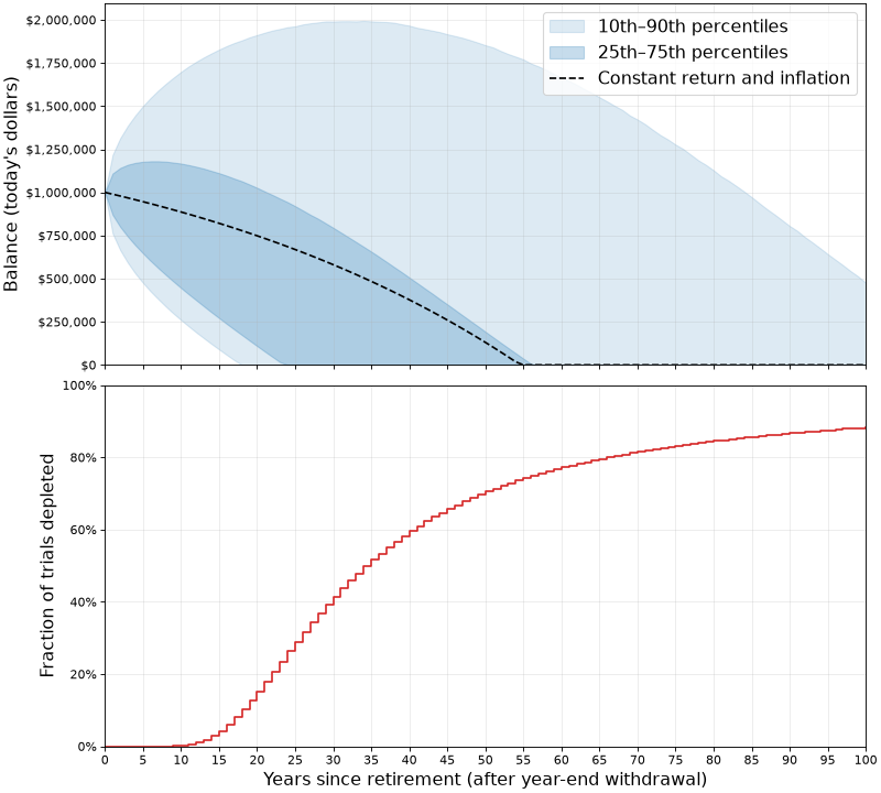
In the top chart:
- The dashed line shows the constant assumptions mentioned before: what happens when yearly return is always 4% and inflation is always 2%.
- The shaded blue areas demonstrate the outcomes of 1,000,000 simulations where inflation and return numbers are drawn from reasonable normal distributions based on historical data. We see that in 25% of the cases, all money ran out by roughly 22 years.
In the bottom chart:
- It's even easier to see how long the funds last; if we're interested in knowing, say, what are the odds that this plan will have enough money for 30 years - the chart shows it's about 60% (since in 40% of the simulations the funds were depleted at this point).
Looking a this simulation, under the current assumptions the plan sounds much riskier than the average assumption makes it appear. Assuming that a 65-y.o. person would plan for 25 years of retirement until death, the ~30% odds of not having sufficient funds for this duration of time are sobering. Perhaps a change in plans is needed (such as a more frugal lifestyle or securing additional funds in some way).
Retirement projection is only one of may ways in which Monte Carlo simulations are used for financial and economical applications; given the high uncertainty of these domains, it's very difficult to plan using analytical calculations. Company sales projections, growth projections, stock offering prices and much more uses Monte Carlo simulations to arrive at estimates with reasonable error bars.
Code
All the code for the explorations in this post is available on GitHub.
| [1] | While these techniques were conceptually understood much earlier, it's not surprising that their first real applications coincided with the development of the first digital computers. As we'll see later in the post, Monte Carlo simulations benefit from running large numbers of trials to get reasonable accuracy. |
| [2] | The answer is: three empty red diamonds, three solid purple ovals, three striped green squiggles. Note that for each of the 4 SET attributes, these three cards are either all the same or all different. |
| [3] | For the same number of trials, this estimate has greater relative uncertainty than the 12-card estimate, because we encounter far fewer hands without a set. |
| [4] | For the examples in this post, we'll be using real dollars, or today's value of the money. We'll assume that the $30,000 yearly draw doesn't change and will instead apply inflation to the portfolio itself. |
| [5] | More sophisticated simulations would let us control these parameters; for example, are the expense funds drawn at the beginning or end of each year, or distributed on a monthly basis? |