When working with multi-dimensional arrays, one important decision programmers have to make fairly early on in the project is what memory layout to use for storing the data, and how to access such data in the most efficient manner. Since computer memory is inherently linear - a one-dimensional structure, mapping multi-dimensional data on it can be done in several ways. In this article I want to examine this topic in detail, talking about the various memory layouts available and their effect on the performance of the code.
Row-major vs. column-major
By far the two most common memory layouts for multi-dimensional array data are row-major and column-major.
When working with 2D arrays (matrices), row-major vs. column-major are easy to describe. The row-major layout of a matrix puts the first row in contiguous memory, then the second row right after it, then the third, and so on. Column-major layout puts the first column in contiguous memory, then the second, etc.
Higher dimensions are a bit more difficult to visualize, so let's start with some diagrams showing how 2D layouts work.
2D row-major
First, some notes on the nomenclature of this article. Computer memory will be represented as a linear array with low addresses on the left and high addresses on the right. Also, we're going to use programmer notation for matrices: rows and columns start with zero, at the top-left corner of the matrix. Row indices go over rows from top to bottom; column indices go over columns from left to right.
As mentioned above, in row-major layout, the first row of the matrix is placed in contiguous memory, then the second, and so on:
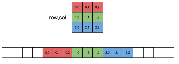
Another way to describe row-major layout is that column indices change the fastest. This should be obvious by looking at the linear layout at the bottom of the diagram. If you read the element index pairs from left to right, you'll notice that the column index changes all the time, and the row index only changes once per row.
For programmers, another important observation is that given a row index
 and a column index
  , the offset of the element
they denote in the linear representation is:
, the offset of the element
they denote in the linear representation is:
![\[offset=i_{row}*NCOLS+i_{col}\]](https://eli.thegreenplace.net/images/math/9161443cbcdff4891bbda9b82127634630ad8952.png)
Where NCOLS is the number of columns per row in the matrix. It's easy to see this equation fits the linear layout in the diagram shown above.
2D column-major
Describing column-major 2D layout is just taking the description of row-major and replacing every appearance of "row" by "column" and vice versa. The first column of the matrix is placed in contiguous memory, then the second, and so on:
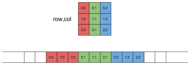
In column-major layout, row indices change the fastest. The offset of an element in column-major layout can be found using this equation:
![\[offset=i_{col}*NROWS+i_{row}\]](https://eli.thegreenplace.net/images/math/ab533f15375dcdb69e7affdd1a4c835e146b7751.png)
Where NROWS is the number of rows per column in the matrix.
Beyond 2D - indexing and layout of N-dimensional arrays
Even though matrices are the most common multi-dimensional arrays programmers deal with, they are by no means the only ones. The notation of multi-dimensional arrays is fully generalizable to more than 2 dimensions. These entities are commonly called "N-D arrays" or "tensors".
When we move to 3D and beyond, it's best to leave the row/column notation of matrices behind. This is because this notation doesn't easily translate to 3 dimensions due to a common confusion between rows, columns and the Cartesian coordinate system. In 4 dimensions and above, we lose any purely-visual intuition to describe multi-dimensional entities anyway, so it's best to stick to a consistent mathematical notation instead.
So let's talk about some arbitrary number of dimensions d, numbered from 1 to
d. For each dimension  ,
,  is the size of the
dimension. Also, the index of an element in dimension
is the size of the
dimension. Also, the index of an element in dimension  is .
For example, in the latest matrix diagram above (where column-layout is shown),
we have
is .
For example, in the latest matrix diagram above (where column-layout is shown),
we have  . If we choose dimension 1 to be the row and dimension 2 to
be the column, then
. If we choose dimension 1 to be the row and dimension 2 to
be the column, then 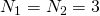 , and the element in the bottom-left corner
of the matrix has
, and the element in the bottom-left corner
of the matrix has  and
and  .
.
In row-major layout of multi-dimensional arrays, the last index is the fastest changing. In case of matrices the last index is columns, so this is equivalent to the previous definition.
Given a  -dimensional array, with the notation shown above, we
compute the memory location of an element from its indices as:
-dimensional array, with the notation shown above, we
compute the memory location of an element from its indices as:
![\[offset=n_d + N_d \cdot (n_{d-1} + N_{d-1} \cdot (n_{d-2} + N_{d-2} \cdot (\cdots + N_2 n_1)\cdots))) = \sum_{i=1}^d \left( \prod_{j=i+1}^d N_j \right) n_i\]](https://eli.thegreenplace.net/images/math/032b2eb5714fa4457fd349eec8f775c3e75584cd.png)
For a matrix, , this reduces to:
![\[offset=n_2 + N_2 \cdot n_1\]](https://eli.thegreenplace.net/images/math/c80b9d7877819556e5059016a2426e9727e0f949.png)
Which is exactly the formula we've seen above for row-major layout, just using a slightly more formal notation.
Similarly, in column-major layout of multi-dimensional arrays, the first index
is the fastest changing. Given a -dimensional array, we compute the
memory location of an element from its indices as:
![\[offset=n_1 + N_1 \cdot (n_2 + N_2 \cdot (n_3 + N_3 \cdot (\cdots + N_{d-1} n_d)\cdots))) = \sum_{i=1}^d \left( \prod_{j=1}^{i-1} N_j \right) n_i\]](https://eli.thegreenplace.net/images/math/35ece5a7b18c317a71e6914ff62c7dd7840952cf.png)
And again, for a matrix with this reduces to the familiar:
![\[offset=n_1+N_1\cdot n_2\]](https://eli.thegreenplace.net/images/math/c084b1f35e57a402567ddc8058ea346d574cd207.png)
Example in 3D
Let's see how this works out in 3D, which we can still visualize. Assuming 3
dimensions: rows, columns and depth. The following diagram shows the memory
layout of a 3D array with 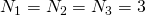 , in row-major:
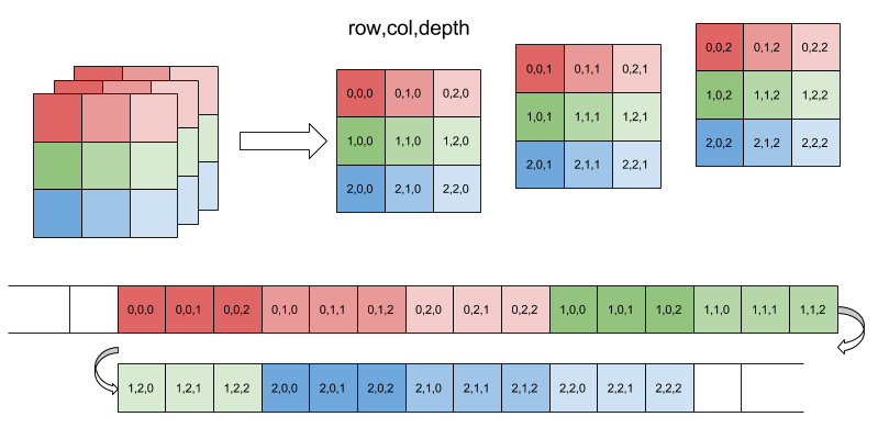
Note how the last dimension (depth, in this case) changes the fastest and the first (row) changes the slowest. The offset for a given element is:
![\[offset=n_3+N_3*(n_2+N_2*n_1)\]](https://eli.thegreenplace.net/images/math/3952a22345f3e71ecbf5b74899d875ca2b9035f2.png)
For example, the offset of the element with indices 2,1,1 is 22.
As an exercise, try to figure out how this array would be laid out in column-major order. But beware - there's a caveat! The term column-major may lead you to believe that columns are the slowest-changing index, but this is wrong. The last index is the slowest changing in column-major, and the last index here is depth, not columns. In fact, columns would be right in the middle in terms of change speed. This is exactly why in the discussion above I suggested dropping the row/column notation when going above 2D. In higher dimensions it becomes confusing, so it's best to refer to the relative change rate of the indices, since these are unambiguous.
In fact, one could conceive a sort of hybrid (or "mixed") layout where the second dimension changes faster than the first or the third. This would be neither row-major nor column-major, but in itself it's a consistent and perfectly valid layout that may benefit some applications. More details on why we would choose one layout over another are later in the article.
History: Fortran vs. C
While knowing which layout a particular data set is using is critical for good performance, there's no single answer to the question which layout "is better" in general. It's not much different from the big-endian vs. little-endian debate; what's important is to pick up a consistent standard and stick to it. Unfortunately, as almost always happens in the world of computing, different programming languages and environments picked different standards.
Among the programming languages still popular today, Fortran was definitely one of the pioneers. And Fortran (which is still very important for scientific computing) uses column-major layout. I read somewhere that the reason for this is that column vectors are more commonly used and considered "canonical" in linear algebra computations. Personally I don't buy this, but you can make your own judgement.
A slew of modern languages follow Fortran's lead - Matlab, R, Julia, to name a few. One of the strongest reasons for this is that they want to use LAPACK - a fast Fortran library for linear algebra, so using Fortran's layout makes sense.
On the other hand, C and C++ use row-major layout. Following their example are a few other popular languages such as Python, Pascal and Mathematica. Since multi-dimensional arrays are a first-class type in the C language, the standard defines the layout very explicitly in section 6.5.2.1 [1].
In fact, having the first index change the slowest and the last index change the fastest makes sense if you think about how multi-dimensional arrays in C are indexed.
Given the declaration:
int x[3][5];
Then x is an array of 3 elements, each of which is an array of 5 integers. x[1] is the address of the second array of 5 integers contained in x, and x[1][4] is the fifth integer of the second 5-integer array in x. These indexing rules imply row-major layout.
None of this is to say that C could not have chosen column-major layout. It could, but then its multi-dimensional array indexing rules would have to be different as well. The result could be just as consistent as what we have now.
Moreover, since C lets you manipulate pointers, you can decide on the layout of data in your program by computing offsets into multi-dimensional arrays on your own. In fact, this is how most C programs are written.
Memory layout example - numpy
So far we've discussed memory layout purely conceptually - using diagrams and mathematical formulae for index computations. It's worthwhile to see a "real" example of how multi-dimensional arrays are stored in memory. For this purpose, the Numpy library of Python is a great tool since it supports both layout kinds and is easy to play with from an interactive shell.
The numpy.array constructor can be used to create multi-dimensional arrays. One of the parameters it accepts is order, which is either "C" for C-style layout (row-major) or "F" for Fortran-style layout (column-major). "C" is the default. Let's see how this looks:
In [42]: ar2d = numpy.array([[1, 2, 3], [11, 12, 13], [10, 20, 40]], dtype='uint8', order='C')
In [43]: '  '.join(str(ord(x)) for x in ar2d.data)
Out[43]: '1  2  3  11  12  13  10  20  40'
In "C" order, elements of rows are contiguous, as expected. Let's try Fortran layout now:
In [44]: ar2df = numpy.array([[1, 2, 3], [11, 12, 13], [10, 20, 40]], dtype='uint8', order='F')

In [45]: '  '.join(str(ord(x)) for x in ar2df.data)
Out[45]: '1  11  10  2  12  20  3  13  40'
For a more complex example, let's encode the following 3D array as a numpy.array and see how it's laid out:
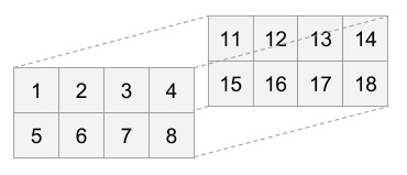
This array has two rows (first dimension), 4 columns (second dimension) and depth 2 (third dimension). As a nested Python list, this is its representation:
In [47]: lst3d = [[[1, 11], [2, 12], [3, 13], [4, 14]], [[5, 15], [6, 16], [7, 17], [8, 18]]]
And the memory layout, in both C and Fortran orders:
In [50]: ar3d = numpy.array(lst3d, dtype='uint8', order='C')

In [51]: '  '.join(str(ord(x)) for x in ar3d.data)
Out[51]: '1  11  2  12  3  13  4  14  5  15  6  16  7  17  8  18'

In [52]: ar3df = numpy.array(lst3d, dtype='uint8', order='F')

In [53]: '  '.join(str(ord(x)) for x in ar3df.data)
Out[53]: '1  5  2  6  3  7  4  8  11  15  12  16  13  17  14  18'
Note that in C layout (row-major), the first dimension (rows) changes the slowest while the third dimension (depth) changes the fastest. In Fortran layout (column-major) the first dimension changes the fastest while the third dimension changes the slowest.
Performance: why it's worth caring which layout your data is in
After reading the article thus far, one may wonder why any of this matters. Isn't it just another way of divergence of standards, a-la endianness? As long as we all agree on the layout, isn't this just a boring implementation detail? Why would we care about this?
The answer is: performance. We're talking about numerical computing here (number crunching on large data sets) where performance is almost always critical. It turns out that matching the way your algorithm works with the data layout can make or break the performance of an application.
The short takeaway is: always traverse the data in the order it was laid out. If your data sits in memory in row-major layout, iterate over each row before going to the next one, etc. The rest of the section will explain why this is so and will also present a benchmask with some measurements to get a feel of the consequences of this decision.
There are two aspects of modern computer architecture that have a large impact on code performance and are relevant to our discussion: caching and vector units. When we iterate over each row of a row-major array, we access the array sequentially. This pattern has spatial locality, which makes the code perfect for cache optimization. Moreover, depending on the operations we do with the data, the CPU's vector unit can kick in since it also requires consecutive access.
Graphically, it looks something like the following diagram. Let's say we have the array: int array[128][128], and we iterate over each row, jumping to the next one when all the columns in the current one were visited. The number within each gray cell is the memory address - it grows by 4 since this is an array if integers. The blue numbered arrow enumerates accesses in the order they are made:
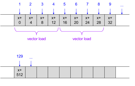
Here, the optimal usage of caching and vector instructions should be obvious. Since we always access elements sequentially, this is the perfect scenario for the CPU's caches to kick in - we will always hit the cache. In fact, we always hit the fastest cache - L1, because the CPU correctly pre-fetches all data ahead.
Moreover, since we always read one 32-bit word [2] after another, we can leverage the CPU's vector units to load the data (and perhaps process is later). The purple arrows show how this can be done with SSE vector loads that grab 128-bit chunks (four 32-bit words) at a time. In actual code, this can either be done with intrinsics or by relying on the compiler's auto-vectorizer (as we will soon see in an actual code sample).
Contrast this with accessing this row-major data one column at a time, iterating over each column before moving to the next one:
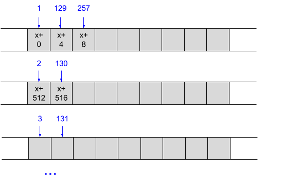
We lose spatial locality here, unless the array is very narrow. If there are few columns, consecutive rows may be found in the cache. However, in more typical applications the arrays are large and when access #2 happens it's likely that the memory it accesses is nowhere to be found in the cache. Unsurprisingly, we also lose the vector units since the accesses are not made to consecutive memory.
But what should you do if your algorithm needs to access data column-by-column rather than row-by-row? Very simple! This is precisely what column-major layout is for. With column-major data, this access pattern will hit all the same architectural sweetspots we've seen with consecutive access on row-major data.
The diagrams above should be convincing enough, but let's do some actual measurements to see just how dramatic these effects are.
The full code for the benchmark is available here, so I'll just show a few selected snippets. We'll start with a basic matrix type laid out in linear memory:
// A simple Matrix of unsigned integers laid out row-major in a 1D array. M is
// number of rows, N is number of columns.
struct Matrix {
  unsigned* data = nullptr;
  size_t M = 0, N = 0;
};
The matrix is using row-major layout: its elements are accessed using this C expression:
x.data[row * x.N + col]
Here's a function that adds two such matrices together, using a "bad" access pattern - iterating over the the rows in each column before going to the next column. The access patter is very easy to spot looking at C code - the inner loop is the faster-changing index, and in this case it's rows:
void AddMatrixByCol(Matrix& y, const Matrix& x) {
  assert(y.M == x.M);
  assert(y.N == x.N);

  for (size_t col = 0; col < y.N; ++col) {
    for (size_t row = 0; row < y.M; ++row) {
      y.data[row * y.N + col] += x.data[row * x.N + col];
    }
  }
}
And here's a version that uses a better pattern, iterating over the columns in each row before going to the next row:
void AddMatrixByRow(Matrix& y, const Matrix& x) {
  assert(y.M == x.M);
  assert(y.N == x.N);

  for (size_t row = 0; row < y.M; ++row) {
    for (size_t col = 0; col < y.N; ++col) {
      y.data[row * y.N + col] += x.data[row * x.N + col];
    }
  }
}
How do the two access patterns compare? Based on the discussion in this article, we'd expect the by-row access pattern to be faster. But how much faster? And what role does vectorization play vs. efficient usage of cache?
To try this, I ran the access patterns on matrices of various sizes, and added a variation of the by-row pattern where vectorization is disabled [3]. Here are the results; the vertical bars represent the bandwidth - how many billions of items (32-bit words) were processed (added) by the given function.
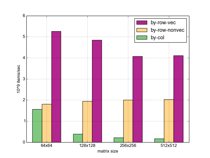
Some observations:
- For matrix sizes above 64x64, by-row access is significantly faster than by-column (6-8x, depending on size). In the case of 64x64, what I believe happens is that both matrices fit into the 32-KB L1 cache of my machine, so the by-column pattern actually manages to find the next row in cache. For larger sizes the matrices no longer fit in L1, so the by-column version has to go to L2 frequently.
- The vectorized version beats the non-vectorized one by 2-3x in all cases. On large matrices the speedup is a bit smaller; I think this is because at 256x256 and beyond the matrices no longer fit in L2 (my machine has 256KB of it) and needs slower memory access. So the CPU spends a bit more time waiting for memory on average.
- The overall speedup of the vectorized by-row access over the by-column access is enormous - up to 25x for large matrices.
I'll have to admit that, while I expected the by-row access to be faster, I didn't expect it to be this much faster. Clearly, choosing the proper access pattern for the memory layout of the data is absolutely crucial for the performance of an application.
Summary
This article examined the issue of multi-dimensional array layout from multiple angles. The main takeaway is: know how your data is laid out and access it accordingly. In C-based programming languages, even though the default layout for 2D-arrays is row-major, when we use pointers to dynamically allocated data, we are free to choose whatever layout we like. After all, multi-dimensional arrays are just a logical abstraction above a linear storage system.
Due to the wonders of modern CPU architectures, choosing the "right" way to access multi-dimensional data may result in colossal speedups; therefore, this is something that should always be on the programmer's mind when working on large multi-dimensional data sets.
| [1] | Taken from draft n1570 of the C11 standard. |
| [2] | The term "word" used to be clearly associated with a 16-bit entity at some point in the past (with "double word" meaning 32 bits and so on), but these days it's too overloaded. In various references online you'll find "word" to be anything from 16 to 64 bits, depending on the CPU architecture. So I'm going to deliberately side-step the confusion by explicitly mentioning the bit size of words. |
| [3] | See the benchmark repository for the full details, including function attributes and compiler flags. A special thanks goes to Nadav Rotem for helping me think through an issue I was initially having due to g++ ignoring my no-tree-vectorize attribute when inlining the function into the benchmark. I turned off inlining to fix this. |