Some notes on implementing attention blocks in pure Python + Numpy. The focus here is on the exact implementation in code, explaining all the shapes throughout the process. The motivation for why attention works is not covered here too deeply - there are plenty of excellent online resources explaining it.
Several papers are mentioned throughout the code; they are:
- AIAYN - Attention Is All You Need by Vaswani et al.
- GPT-3 - Language Models are Few-Shot Learners by Brown et al.
Basic scaled self-attention
We'll start with the most basic scaled dot product self-attention, working on a single sequence of tokens, without masking.
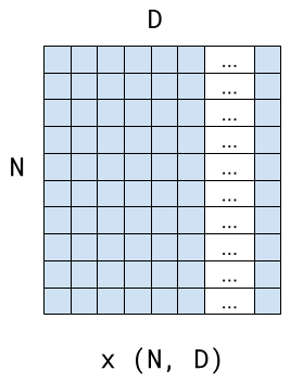
The input is a 2D array of shape (N, D). N is the length of the sequence (how many tokens it contains) and D is the embedding depth - the length of the embedding vector representing each token [1]. D could be something like 512, or more, depending on the model.
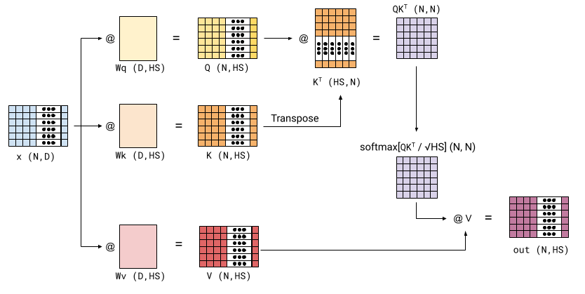
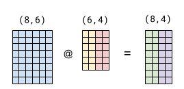
A self-attention module is parameterized with three weight matrices, Wk, Wq and Wv. Some variants also have accompanying bias vectors, but the AIAYN paper doesn't use them, so I'll skip them here. In the general case, the shape of each weight matrix is (D, HS), where HS is some fraction of D. HS stands for "head size" and we'll see what this means soon. This is a diagram of a self-attention module (the diagram assumes N=6, D is some large number and so is HS). In the diagram, @ stands for matrix multiplication (Python/Numpy syntax):
Here's a basic Numpy implementation of this:
# self_attention the way it happens in the Transformer model. No bias.
# D = model dimension/depth (length of embedding)
# N = input sequence length
# HS = head size
#
# x is the input (N, D), each token in a row.
# Each of W* is a weight matrix of shape (D, HS)
# The result is (N, HS)
def self_attention(x, Wk, Wq, Wv):
    # Each of these is (N, D) @ (D, HS) = (N, HS)
    q = x @ Wq
    k = x @ Wk
    v = x @ Wv

    # kq: (N, N) matrix of dot products between each pair of q and k vectors.
    # The division by sqrt(HS) is the scaling.
    kq = q @ k.T / np.sqrt(k.shape[1])

    # att: (N, N) attention matrix. The rows become the weights that sum
    # to 1 for each output vector.
    att = softmax_lastdim(kq)
    return att @ v  # (N, HS)
The "scaled" part is just dividing kq by the square root of HS, which is done to keep the values of the dot products manageable (otherwise they would grow with the size of the contracted dimension).
The only dependency is a function for calculating Softmax across the last dimension of an input array:
def softmax_lastdim(x):
    """Compute softmax across last dimension of x.

    x is an arbitrary array with at least two dimensions. The returned array has
    the same shape as x, but its elements sum up to 1 across the last dimension.
    """
    # Subtract the max for numerical stability
    ex = np.exp(x - np.max(x, axis=-1, keepdims=True))
    # Divide by sums across last dimension
    return ex / np.sum(ex, axis=-1, keepdims=True)
When the input is 2D, the "last dimension" is the columns. Colloquially, this Softmax function acts on each row of x separately; it applies the Softmax formula to the elements (columns) of the row, ending up with a row of numbers in the range [0,1] that all sum up to 1.
Another note on the dimensions: it's possible for the Wv matrix to have a different second dimension from Wq and Wk. If you look at the diagram, you can see this will work out, since the softmax produces (N, N), and whatever the second dimension of V is, will be the second dimension of the output. The AIAYN paper designates these dimensions as and , but in practice in all the variants it lists. I found that these dimensions are typically the same in other papers as well. Therefore, for simplicity I just made them all equal to D in this post; if desired, a variant with different and is a fairly trivial modification to this code.
Batched self-attention
In the real world, the input array is unlikely to be 2D because models are trained on batches of input sequences. To leverage the parallelism of modern hardware, whole batches are typically processed in the same operation.
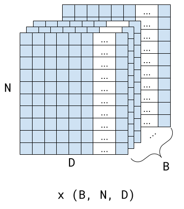
The batched version of scaled self-attention is very similar to the non-batched one, due to the magic of Numpy matrix multiplication and broadcasts. Now the input shape is (B, N, D), where B is the batch dimension. The W* matrices are still (D, HS); multiplying a (B, N, D) array by (D, HS) performs contraction between the last axis of the first array and the first axis of the second array, resulting in (B, N, HS). Here's the code, with the dimensions annotated for each operation:
# self_attention with inputs that have a batch dimension.
# x has shape (B, N, D)
# Each of W* has shape (D, D)
def self_attention_batched(x, Wk, Wq, Wv):
    q = x @ Wq  # (B, N, HS)
    k = x @ Wk  # (B, N, HS)
    v = x @ Wv  # (B, N, HS)

    kq = q @ k.swapaxes(-2, -1) / np.sqrt(k.shape[-1])  # (B, N, N)

    att = softmax_lastdim(kq)  # (B, N, N)
    return att @ v  # (B, N, HS)
Note that the only difference between this and the non-batched version is the line calculating kq:
- Since k is no longer 2D, the notion of "transpose" is ambiguous so we explicitly ask to swap the last and the penultimate axis, leaving the first axis (B) intact.
- When calculating the scaling factor we use k.shape[-1] to select the last dimension of k, instead of k.shape[1] which only selects the last dimension for 2D arrays.
In fact, this function could also calculate the non-batched version! From now on, we'll assume that all inputs are batched, and all operations are implicitly batched. I'm not going to be using the "batched" prefix or suffix on functions any more.
The basic underlying idea of the attention module is to shift around the multi-dimensional representations of tokens in the sequence towards a better representation of the entire sequence. The tokens attend to each other. Specifically, the matrix produced by the Softmax operation is called the attention matrix. It's (N, N); for each token it specifies how much information from every other token in the sequence should be taken into account. For example, a higher number in cell (R, C) means that there's a stronger relation of token at index R in the sequence to the token at index C.
Here's a nice example from the AIAYN paper, showing a word sequence and the weights produced by two attention heads (purple and brown) for a given position in the input sequence:
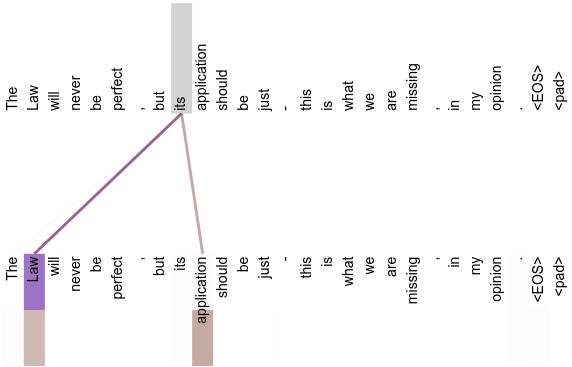
This shows how the model is learning to resolve what the word "its" refers to in the sentence. Let's take just the purple head as an example. The index of token "its" in the sequence is 8, and the index of "Law" is 1. In the attention matrix for this head, the value at index (8, 1) will be very high (close to 1), with other values in the same row much lower.
While this intuitive explanation isn't critical to understand how attention is implemented, it will become more important when we talk about masked self-attention later on.
Multi-head attention
The attention mechanism we've seen so far has a single set of K, Q and V matrices. This is called one "head" of attention. In today's models, there are typically multiple heads. Each head does its attention job separately, and in the end all these results are concatenated and feed through a linear layer.
In what follows, NH is the number of heads and HS is the head size. Typically, NH times HS would be D; for example, the AIAYN paper mentions several configurations for D=512: NH=8 and HS=64, NH=32 and HS=16, and so on [2]. However, the math works out even if this isn't the case, because the final linear ("projection") layer maps the output back to (N, D).
Assuming the previous diagram showing a self-attention module is a single head with input (N, D) and output (N, HS), this is how multiple heads are combined:
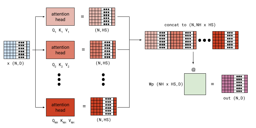
Each of the (NH) heads has its own parameter weights for Q, K and V. Each attention head outputs a (N, HS) matrix; these are concatenated along the last dimension to (N, NH * HS), which is passed through a final linear projection.
Here's a function implementing (batched) multi-head attention; for now, please ignore the code inside do_mask conditions:
# x has shape (B, N, D)
# In what follows:
#   NH = number of heads
#   HS = head size
# Each W*s is a list of NH weight matrices of shape (D, HS).
# Wp is a weight matrix for the final linear projection, of shape (NH * HS, D)
# The result is (B, N, D)
# If do_mask is True, each attention head is masked from attending to future
# tokens.
def multihead_attention_list(x, Wqs, Wks, Wvs, Wp, do_mask=False):
    # Check shapes.
    NH = len(Wks)
    HS = Wks[0].shape[1]
    assert len(Wks) == len(Wqs) == len(Wvs)
    for W in Wqs + Wks + Wvs:
        assert W.shape[1] == HS
    assert Wp.shape[0] == NH * HS

    # List of head outputs
    head_outs = []

    if do_mask:
        # mask is a lower-triangular (N, N) matrix, with zeros above
        # the diagonal and ones on the diagonal and below.
        N = x.shape[1]
        mask = np.tril(np.ones((N, N)))

    for Wk, Wq, Wv in zip(Wks, Wqs, Wvs):
        # Calculate self attention for each head separately
        q = x @ Wq  # (B, N, HS)
        k = x @ Wk  # (B, N, HS)
        v = x @ Wv  # (B, N, HS)

        kq = q @ k.swapaxes(-2, -1) / np.sqrt(k.shape[-1])  # (B, N, N)

        if do_mask:
            # Set the masked positions to -inf, to ensure that a token isn't
            # affected by tokens that come after it in the softmax.
            kq = np.where(mask == 0, -np.inf, kq)

        att = softmax_lastdim(kq)  # (B, N, N)
        head_outs.append(att @ v)  # (B, N, HS)

    # Concatenate the head outputs and apply the final linear projection
    all_heads = np.concatenate(head_outs, axis=-1)  # (B, N, NH * HS)
    return all_heads @ Wp  # (B, N, D)
It is possible to vectorize this code even further; you'll sometimes see the heads laid out in a separate (4th) dimension instead of being a list. See the Vectorizing across the heads dimension section.
Masked (or Causal) self-attention
Attention modules can be used in both encoder and decoder blocks. Encoder blocks are useful for things like language understanding or translation; for these, it makes sense for each token to attend to all the other tokens in the sequence.
However, for generative models this presents a problem: if during training a word attends to future words, the model will just "cheat" and not really learn how to generate the next word from only past words. This is done in a decoder block, and for this we need to add masking to attention.
Conceptually, masking is very simple. Consider the sentence:
People like watching funny cat videos
When our attention code generates the att matrix, it's a square (N, N) matrix with attention weights from each token to each other token in the sequence:
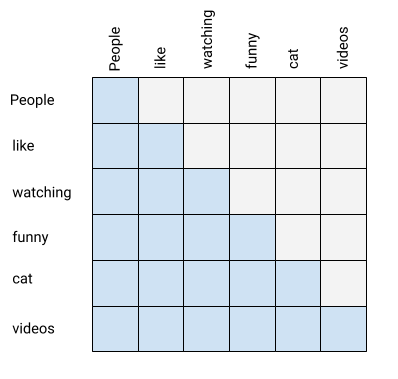
What we want is for all the gray cells in this matrix to be zero, to ensure that a token doesn't attend to future tokens. The blue cells in the matrix add up to 1 in each row, after the softmax operation.
Now take a look at the previous code sample and see what happens when do_mask=True:
- First, a (N, N) lower-triangular array is prepared with zeros above the diagonal and ones on the diagonal and below.
- Then, before we pass the scaled to softmax, we set its values to wherever the mask matrix is 0. This ensures that the softmax function will assign zeros to outputs at these indices, while still producing the proper values in the rest of the row.
Another name for masked self-attention is causal self-attention. This is a very good name that comes from causal systems in control theory.
Intuition - what attention does
What does the attention block try to accomplish? To think about it intuitively, let's focus on a single token in the input (ignoring batch) - x[i]. For this token, the attention block produces an output token out[i] that blends x[i]'s embedding (multi-dimensional dense vector representation) with contextual information from all the tokens preceding it in the sequence, i.e. x[:i].
The way this is done is first calculating the query vector q for x[i] (using Wq). This query can be thought of as "what attributes does this token care about in its context tokens".
Then, for each of the context tokens (including x[i] itself) we calculate:
- Key (using Wk): these are the attributes of the token that queries may refer to.
- Value (using Wv): these are the associated values tokens carry.
When attention calculates q @ K.T for each token, the result is - for each context token - the weights to use for mixing in the token's value. Then, when this is multiplied by V, the values are properly weighted.
So this is a very general approach for the model to learn what kind of information each token "cares" about in its context tokens, and how to blend the token's embedding with those of the preceding context tokens, to properly encode the context the token is encountered in.
Our implementation, starting with the basic scaled self-attention, implements this for all tokens in the input sequence simultaneously; hence, we don't just take a single x[i], calculate its q and then multiply that by K.T. Rather, we calculate Q from all x, and continue using matrix multiplications to vectorize these calculations across the entire sequence.
It's important to keep in mind that this intuitive explanation suffers from anthropomorphism. We try to explain what the model does intuitively, but in reality this is only a very abstract approximation of what's happening (consider that attention has multiple heads, and also that that LLMs typically have dozens of repeating transformer layers with self-attention blocks, applying the same mechanism over and over again).
Cross-attention
So far we've been working with self-attention blocks, where the self suggests that elements in the input sequence attend to other elements in the same input sequence.
Another variant of attention is cross-attention, where elements of one sequence attend to elements in another sequence. This variant exists in the decoder block of the AIAYN paper. This is a single head of cross-attention:
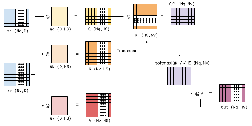
Here we have two sequences with potentially different lengths: xq and xv. xq is used for the query part of attention, while xv is used for the key and value parts. The rest of the dimensions remain as before. The output of such a block is shaped (Nq, HS).
This is an implementation of multi-head cross-attention; it doesn't include masking, since masking is not typically necessary in cross attention - it's OK for elements of xq to attend to all elements of xv [3]:
# Cross attention between two input sequences that can have different lengths.
# xq has shape (B, Nq, D)
# xv has shape (B, Nv, D)
# In what follows:
#   NH = number of heads
#   HS = head size
# Each W*s is a list of NH weight matrices of shape (D, HS).
# Wp is a weight matrix for the final linear projection, of shape (NH * HS, D)
# The result is (B, Nq, D)
def multihead_cross_attention_list(xq, xv, Wqs, Wks, Wvs, Wp):
    # Check shapes.
    NH = len(Wks)
    HS = Wks[0].shape[1]
    assert len(Wks) == len(Wqs) == len(Wvs)
    for W in Wqs + Wks + Wvs:
        assert W.shape[1] == HS
    assert Wp.shape[0] == NH * HS

    # List of head outputs
    head_outs = []

    for Wk, Wq, Wv in zip(Wks, Wqs, Wvs):
        q = xq @ Wq  # (B, Nq, HS)
        k = xv @ Wk  # (B, Nv, HS)
        v = xv @ Wv  # (B, Nv, HS)

        kq = q @ k.swapaxes(-2, -1) / np.sqrt(k.shape[-1])  # (B, Nq, Nv)

        att = softmax_lastdim(kq)  # (B, Nq, Nv)
        head_outs.append(att @ v)  # (B, Nq, HS)

    # Concatenate the head outputs and apply the final linear projection
    all_heads = np.concatenate(head_outs, axis=-1)  # (B, Nq, NH * HS)
    return all_heads @ Wp  # (B, Nq, D)
Vectorizing across the heads dimension
The multihead_attention_list implementation shown above uses lists of weight matrices as input. While this makes the code clearer, it's not a particularly friendly format for an optimized implementation - especially on accelerators like GPUs and TPUs. We can vectorize it further by creating a new dimension for attention heads.
To understand the trick being used, consider a basic matmul of (8, 6) by (6, 2):
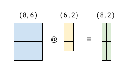
Now suppose we want to multiply our LHS by another (6, 2) matrix. We can do it all in the same operation by concatenating the two RHS matrices along columns:
If the yellow RHS block in both diagrams is identical, the green block of the result will be as well. And the violet block is just the matmul of the LHS by the red block of the RHS. This stems from the semantics of matrix multiplication, and is easy to verify on paper.
Now back to our multi-head attention. Note that we multiply the input x by a whole list of weight matrices - in fact, by three lists (one list for Q, one for K, and another for V). We can use the same vectorization technique by concatenating all these weight matrices into a single one. Assuming that NH * HS = D, the shape of the combined matrix is (D, 3 * D). Here's the vectorized implementation:
# x has shape (B, N, D)
# In what follows:
#   NH = number of heads
#   HS = head size
#   NH * HS = D
# W is expected to have shape (D, 3 * D), with all the weight matrices for
# Qs, Ks, and Vs concatenated along the last dimension, in this order.
# Wp is a weight matrix for the final linear projection, of shape (D, D).
# The result is (B, N, D).
# If do_mask is True, each attention head is masked from attending to future
# tokens.
def multihead_attention_vec(x, W, NH, Wp, do_mask=False):
    B, N, D = x.shape
    assert W.shape == (D, 3 * D)
    qkv = x @ W  # (B, N, 3 * D)
    q, k, v = np.split(qkv, 3, axis=-1)  # (B, N, D) each

    if do_mask:
        # mask is a lower-triangular (N, N) matrix, with zeros above
        # the diagonal and ones on the diagonal and below.
        mask = np.tril(np.ones((N, N)))

    HS = D // NH
    q = q.reshape(B, N, NH, HS).transpose(0, 2, 1, 3)  # (B, NH, N, HS)
    k = k.reshape(B, N, NH, HS).transpose(0, 2, 1, 3)  # (B, NH, N, HS)
    v = v.reshape(B, N, NH, HS).transpose(0, 2, 1, 3)  # (B, NH, N, HS)

    kq = q @ k.swapaxes(-1, -2) / np.sqrt(k.shape[-1])  # (B, NH, N, N)

    if do_mask:
        # Set the masked positions to -inf, to ensure that a token isn't
        # affected by tokens that come after it in the softmax.
        kq = np.where(mask == 0, -np.inf, kq)

    att = softmax_lastdim(kq)  # (B, NH, N, N)
    out = att @ v  # (B, NH, N, HS)
    return out.transpose(0, 2, 1, 3).reshape(B, N, D) @ Wp  # (B, N, D)
This code computes Q, K and V in a single matmul, and then splits them into separate arrays (note that on accelerators these splits and later transposes may be very cheap or even free as they represent a different access pattern into the same data).
Each of Q, K and V is initially (B, N, D), so they are reshaped into a more convenient shape by first splitting the D into (NH, HS), and finally changing the order of dimensions to get (B, NH, N, HS). In this format, both B and NH are considered batch dimensions that are fully parallelizable. The computation can then proceed as before, and Numpy will automatically perform the matmul over all the batch dimensions.
Sometimes you'll see an alternative notation used in papers for these matrix multiplications: numpy.einsum. For example, in our last code sample the computation of kq could also be written as:
kq = np.einsum("bhqd,bhkd->bhqk", q, k) / np.sqrt(k.shape[-1])
Code
The full code for these samples, with tests, is available in this repository.
| [1] | In LLM papers, D is often called . |
| [2] | In the GPT-3 paper, this is also true for all model variants. For example, the largest 175B model has NH=96, HS=128 and D=12288. |
| [3] | It's also not as easy to define mathematically: how do we make a non-square matrix triangular? And what does it mean when the lengths of the two inputs are different? |