Cross-entropy and KL divergence

Information content of a single random event

We'll start with a single event (E) that has probability p. The information content (or "degree of surprise") of this event occurring is defined as:

The base 2 here is used so that we can count the information in units of bits. Thinking about this definition intuitively, imagine an event with probability p=1; using the formula, the information we gain by observing this event occurring is 0, which makes sense. On the other extreme, as the probability p approaches 0, the information we gain is huge. An equivalent way to write the formula is:

Some numeric examples: suppose we flip a fair coin and it comes out heads. The probability of this event happening is 1/2, therefore:

Now suppose we roll a fair die and it lands on 4. The probability of this event happening is 1/6, therefore:

In other words, the degree of surprise for rolling a 4 is higher than the degree of surprise for flipping to heads - which makes sense, given the probabilities involved.

Other than behaving correctly for boundary values, the logarithm function makes sense for calculating the degree of surprise for another important reason: the way it behaves for a combination of events.

Consider this: we flip a fair coin and roll a fair die; the coin comes out heads, and the die lands on 4. What is the probability of this event happening? Because the two events are independent, the probability is the product of the probabilities of the individual events, so 1/12, and then:

Note that the entropy is the precise sum of the entropies of individual events. This is to be expected - we need so many bits for one of the events, and so many for the other; the total of the bits adds up. The logarithm function gives us exactly this behavior for probabilities:

Entropy

Given a random variable X with values and associated probabilities , the entropy of X is defined as the expected value of information for X:

High entropy means high uncertainty, while low entropy means low uncertainty. Let's look at a couple of examples:

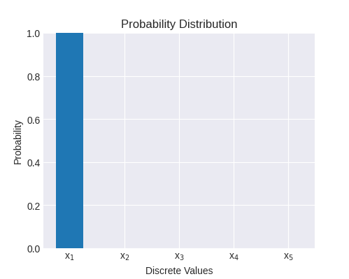
This is a random variable with 5 distinct values; the probability of is 1, and the rest is 0. The entropy here is 0, because and also [1]. We gain no information by observing an event sampled from this distribution, because we knew ahead of time what would happen.

Another example is a uniform distribution for the 5 possible outcomes:

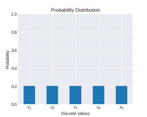
The entropy for this distribution is:

Intuitively: we have 5 different values with equal probabilities, so we'll need bits to represent that. Note that entropy is always non-negative, because and therefore for all j in a proper probability distribution.

It's not hard to show that the maximum possible entropy for a random variable occurs for a uniform distribution. In all other distributions, some values are more represented than others which makes the result somewhat less surprising.

Cross-entropy

Cross-entropy is an extension of the concept of entropy, when two different probability distributions are present. The typical formulation useful for machine learning is:

Where:

• P is the actual observed data distribution
• Q is the predicted data distribution

Similarly to entropy, cross-entropy is non-negative; in fact, it collapses to the entropy formula when P and Q are the same:

An information-theoretic interpretation of cross-entropy is: the average number of bits required to encode an actual probability distribution P, when we assumed the data follows Q instead.

Here's a numeric example:

p = [0.1, 0.2, 0.4, 0.2, 0.1]
q = [0.2, 0.2, 0.2, 0.2, 0.2]

Plotted:

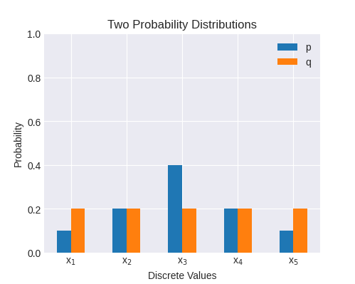
The cross-entropy of these two distributions is 2.32

Now let's try a Q that's slightly closer to P:

p = [0.1, 0.2, 0.4, 0.2, 0.1]
q = [0.15, 0.175, 0.35, 0.175, 0.15]

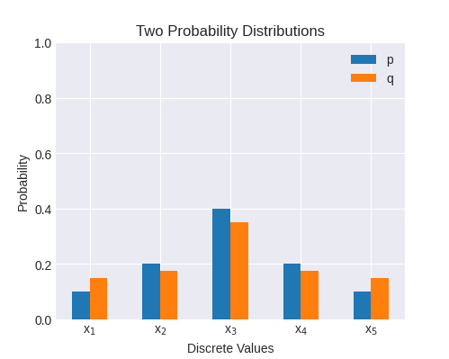
The cross-entropy in these distributions is somewhat lower, 2.16; this is expected, because they're more similar. In other words, the outcome of measuring P when our model predicted Q is less surprising.

KL divergence

Cross-entropy is useful for tracking the training loss of a model (more on this in the next section), but it has some mathematical properties that make it less than ideal as a statistical tool to compare two probability distributions. Specifically, , which isn't (usually) zero; this is the lowest value possible for cross-entropy. In other words, cross-entropy always retains the inherent uncertainty of P.

The KL divergence fixes this by subtracting from cross-entropy:

Manipulating the logarithms, we can also get these alternative formulations:

Thus, the KL divergence is more useful as a measure of divergence between two probability distributions, since . Note, however, that it's not a true distance metric because it's not symmetric:

Uses in machine learning

In ML, we often have a model that makes a prediction and a set of training data which defines a real-world probability distribution. It's natural to define a loss function in terms of the difference between the two distributions (the model's prediction and the real data).

Cross-entropy is very useful as a loss function because it's non-negative and provides a single scalar number that's lower for similar distributions and higher for dissimilar distributions. Moreover, if we think of cross-entropy in terms of KL divergence:

We'll notice that - the entropy of the real-world distribution - does not depend on the model at all. Therefore, optimizing cross-entropy is equivalent to optimizing the KL divergence. I wrote about concrete uses of cross-entropy as a loss function in previous posts:

• Logistic regression
• Softmax for multiclass classification

That said, the KL divergence is also sometimes useful more directly; for example in the evidence lower bound used for Variational autoencoders.

Relation to Maximum Likelihood Estimation

There's an interesting relation between the concepts discussed in this post and Maximum Likelihood Estimation.

Suppose we have a true probability distribution P, and a parameterized model that predicts the probability distribution . stands for all the parameters of our model (e.g. all the weights of a deep learning network).

The likelihood of observing a set of samples drawn from P is:

However, we don't really know P; what we do know is , so we can calculate:

The idea is to find an optimal set of parameters such that this likelihood is maximized; in other words:

Working with products is inconvenient, however, so a logarithm is used instead to convert a product to a sum (since is a monotonically increasing function, maximizing it is akin to maximizing itself):

This is the maximal log-likelihood.

Now a clever statistical trick is employed; first, we multiply the function we're maximizing by the constant - this doesn't affect the maxima, of course:

The function inside the argmax is now the average across n samples obtained from the true probability distribution P. The Law of Large numbers states that with a large enough n, this average converges to the expected value of drawing from this distribution:

This should start looking familiar; all that's left is to negate the sum and minimize the negative instead:

The function we're now minimizing is the cross-entropy between P and . We've shown that maximum likelihood estimation is equivalent to minimizing the cross-entropy between the true and and predicted data distributions.