The goal of this post is to answer a simple question: why are the following two definitions of the vector dot product in Euclidean space [1] equivalent for vectors and :
- Component definition:
- Geometric definition:
, where
is the magnitude of and
 is the angle between the vectors’ directions
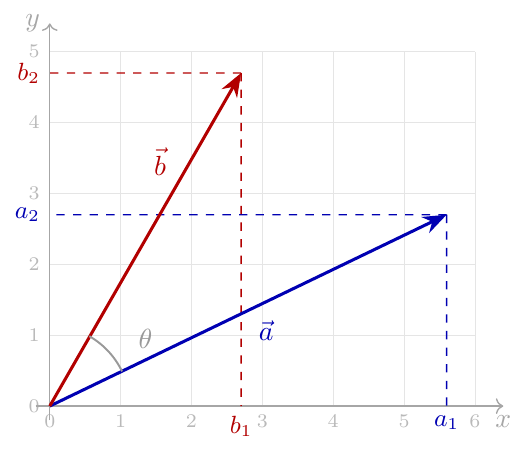
Here’s a graphical depiction of our vectors (focusing on
 for clarity, though this applies to any-dimensional
vectors). It shows both the components of the vectors and the angle
between them. The length of the arrow for is
.
for clarity, though this applies to any-dimensional
vectors). It shows both the components of the vectors and the angle
between them. The length of the arrow for is
.
We’ll show two proofs of the equivalence here, the geometric proof and the projection proof. The Appendix describes some properties of dot products that facilitate these proofs.
Geometric proof
We’ll be using this diagram of our vectors and , as well as the vector :
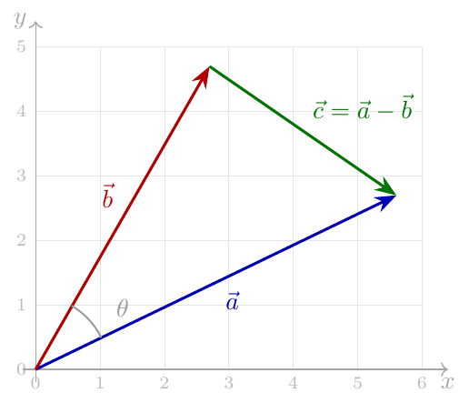
Using the law of cosines [2] on the triangle formed by the three vectors:
Since for any vector , we have (see Appendix), let’s rewrite this equation as:
But and the dot product obeys the distributive property (see Appendix). Therefore:
Projection proof
For this proof, we’ll assume the geometric definition is correct and
will see how it leads to the component definition. We’ll begin by
denoting vectors as the
standard orthonormal basis for  . For example, in 2D
space, these basis vectors are and
, shown in
this diagram:
. For example, in 2D
space, these basis vectors are and
, shown in
this diagram:
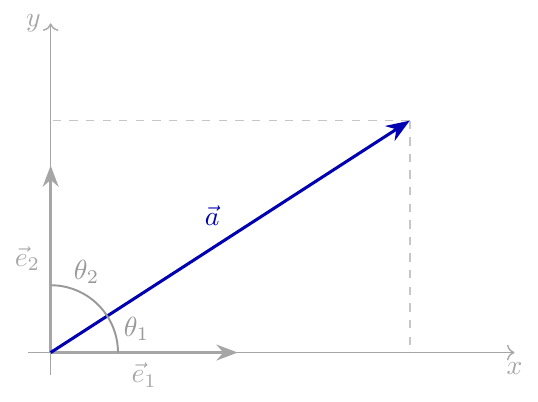
If we take an arbitrary and calculate its dot product with a basis vector, we can use the geometric definition:
where is the component of in the direction of . The diagram makes it easy to see why this is true from basic trigonometry, but in the more general case this is just a vector projection.
Now let’s represent vectors and as linear combinations of the basis vectors:
And calculate the dot product , beginning by rewriting with its linear combination of basis vectors representation:
Using the fact that the dot product distributes over linear combinations:
But earlier we’ve shown that . Therefore:
Which is the component definition .
Appendix A: Inner product space
A generalization of dot products in is the inner
product, which is an operation meeting some specific requirements,
defined on a vector space.
The inner product is denoted as , and must satisfy the following requirements for all vectors and scalars :
- Symmetry:
- Linearity in the first argument:
- Positive-definiteness: if then
For , we define the inner product operation in its
component formulation as:
Let’s prove the requirements listed above for this operation; this is
fairly straightforward, given the well-known properties of scalar
multiplication and addition on  :
:
Symmetry:
Linearity in the first argument:
Positive-definiteness:
Consider the components  of vector . Clearly,
. Since the vector
is not the zero vector, at least one of its components
is nonzero, and for that component .
Therefore:
of vector . Clearly,
. Since the vector
is not the zero vector, at least one of its components
is nonzero, and for that component .
Therefore:
Now that we’ve proved all the inner product requirements on our
operation , we can say that
is an inner product space with this operation.
By meeting these requirements, it can be readily shown that our inner product operation has additional useful properties:
- if and only if
The third property is particularly helpful, because it means the inner product is bilinear, and thus is distributive over addition.
Note that these are shown for the component definition of dot product. It’s not too hard to prove distributivity for the geometric definition using the notion of projections and how they add up.
Norm
The norm of a vector in an inner product space is defined as . Therefore, the square of the norm is .
The norm is used to express the notion of magnitude, or length of a vector. If you think of a vector in Cartesian coordinates, the definition of the norm is a generalization of the Pythagorean theorem.
| [1] | By this we mean , where each vector is an n-tuple
of real numbers, with the usual mathematical operations making this a
vector space. |
| [2] | Which is a very fundamental theorem in geometry; it is (or rather, its non-trigonometric version) is proven from the basic Euclidean axioms in The Elements. |