When traversing trees with DFS, orderings are easy to define: we have pre-order, which visits a node before recursing into its children; in-order, which visits a node in-between recursing into its children; post-order, which visits a node after recursing into its children.
However, for directed graphs, these orderings are not as natural and slightly different definitions are used. In this article I want to discuss the various directed graph orderings and their implementations. I also want to mention some applications of directed graph traversals to data-flow analysis.
Directed graphs are my focus here, since these are most useful in the applications I'm interested in. When a directed graph is known to have no cycles, I may refer to it as a DAG (directed acyclic graph). When cycles are allowed, undirected graphs can be simply modeled as directed graphs where each undirected edge turns into a pair of directed edges.
Depth-first search and pre-order
Let's start with the basis algorithm for everything discussed in this article - depth-first search (DFS). Here is a simple implementation of DFS in Python (the full code is available here):
def dfs(graph, root, visitor):
    """DFS over a graph.

    Start with node 'root', calling 'visitor' for every visited node.
    """
    visited = set()
    def dfs_walk(node):
        visited.add(node)
        visitor(node)
        for succ in graph.successors(node):
            if not succ in visited:
                dfs_walk(succ)
    dfs_walk(root)
This is the baseline implementation, and we'll see a few variations on it to implement different orderings and algorithms. You may think that, due to the way the algorithm is structured, it implements pre-order traversal. It certainly looks like it. In fact, pre-order traversal on graphs is defined as the order in which the aforementioned DFS algorithm visited the nodes. However, there's a subtle but important difference from tree pre-order. Whereas in trees, we may assume that in pre-order traversal we always see a node before all its successors, this isn't true for graph pre-order. Consider this graph:
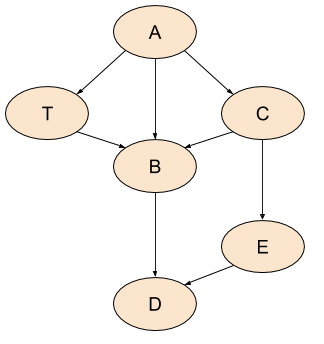
If we print the nodes in the order visited by DFS, we may get something like: A, C, B, D, E, T. So B comes before T, even though B is T's successor [1].
We'll soon see that other orderings do provide some useful guarantees.
Post-order and reverse post-order
To present other orderings and algorithms, we'll take the dfs function above and tweak it slightly. Here's a post-order walk. It has the same general structure as dfs, but it manages additional information (order list) and doesn't call a visitor function:
def postorder(graph, root):
    """Return a post-order ordering of nodes in the graph."""
    visited = set()
    order = []
    def dfs_walk(node):
        visited.add(node)
        for succ in graph.successors(node):
            if not succ in visited:
                dfs_walk(succ)
        order.append(node)
    dfs_walk(root)
    return order
This algorithm adds a node to the order list when its traversal is fully finished; that is, when all its outgoing edges have been visited. Unlike pre-order, here it's actually ensured - in the absence of cycles - that for two nodes V and W, if there is a path from W to V in the graph, then V comes before W in the list [2].
Reverse post-order (RPO) is exactly what its name implies. It's the reverse of the list created by post-order traversal. In reverse post-order, if there is a path from V to W in the graph, V appears before W in the list. Note that this is actually a useful guarantee - we see a node before we see any other nodes reachable from it; for this reason, RPO is useful in many algorithms.
Let's see the orderings produced by pre-order, post-order and RPO for our sample DAG:
- Pre-order: A, C, B, D, E, T
- Post-order: D, B, E, C, T, A
- RPO: A, T, C, E, B, D
This example should help dispel a common confusion about these traversals - RPO is not the same as pre-order. While pre-order is simply the order in which DFS visits a graph, RPO actually guarantees that we see a node before all of its successors (again, this is in the absence of cycles, which we'll deal with later). So if you have an algorithm that needs this guarantee and you could simply use pre-order on trees, when you're dealing with DAGs it's RPO, not pre-order, that you're looking for.
Topological sort
In fact, the RPO of a DAG has another name - topological sort. Indeed, listing a DAG's nodes such that a node comes before all its successors is precisely what sorting it topologically means. If nodes in the graph represent operations and edges represent dependencies between them (an edge from V to W meaning that V must happen before W) then topological sort gives us an order in which we can run the operations such that all the dependencies are satisfied (no operation runs before its dependencies).
DAGs with multiple roots
So far the examples and algorithms demonstrated here show graphs that have a single, identifiable root node. This is not always the case for realistic graphs, though it is most likely the case for graphs used in compilation because a program has a single entry function (for call graphs) and a function has a single entry instruction or basic block (for control-flow and data-flow analyses of functions).
Once we leave the concept of "one root to rule them all" behind, it's not even clear how to traverse a graph like the example used in the article so far. Why start from node A? Why not B? And how would the traversal look if we did start from B? We'd then only be able to discover B itself and D, and would have to restart to discover other nodes.
Here's another graph, where not all nodes are connected with each other. This graph has no pre-defined root [3]. How do we still traverse all of it in a meaningful way?
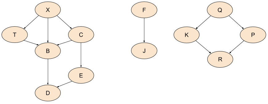
The idea is a fairly simple modification of the DFS traversal shown earlier. We pick an arbitrary unvisited node in the graph, treat it as a root and start dutifully traversing. When we're done, we check if there are any unvisited nodes remaining in the graph. If there are, we pick another one and restart. So on and so forth until all the nodes are visited:
def postorder_unrooted(graph):
    """Unrooted post-order traversal of a graph.

    Restarts traversal as long as there are undiscovered nodes. Returns a list
    of lists, each of which is a post-order ordering of nodes discovered while
    restarting the traversal.
    """
    allnodes = set(graph.nodes())
    visited = set()
    orders = []
    def dfs_walk(node):
        visited.add(node)
        for succ in graph.successors(node):
            if not succ in visited:
                dfs_walk(succ)
        orders[-1].append(node)
    while len(allnodes) > len(visited):
        # While there are still unvisited nodes in the graph, pick one at random
        # and restart the traversal from it.
        remaining = allnodes - visited
        root = remaining.pop()
        orders.append([])
        dfs_walk(root)
    return orders
To demonstrate this approach, postorder_unrooted returns not just a single list of nodes ordered in post-order, but a list of lists. Each list is a post-order ordering of a set of nodes that were visited together in one iteration of the while loop. Running on the new sample graph, I get this:
[
 ['d', 'b', 'e', 'c'],
 ['j', 'f'],
 ['r', 'k'],
 ['p', 'q'],
 ['t', 'x']
]
There's a slight problem with this approach. While relative ordering between entirely unconnected pieces of the graph (like K and and X) is undefined, the ordering within each connected piece may be defined. For example, even though we discovered T and X separately from D, B, E, C, there is a natural ordering between them. So a more sophisticated algorithm would attempt to amend this by merging the orders when that makes sense. Alternatively, we can look at all the nodes in the graph, find the ones without incoming edges and use these as roots to start from.
Directed graphs with cycles
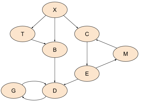
Cycles in directed graphs present a problem for many algorithms, but there are important applications where avoiding cycles is unfeasible, so we have to deal with them. Here's a sample graph with a couple of cycles:
Cycles break almost all of the nice-and-formal definitions of traversals stated so far in the article. In a graph with cycles, there is - by definition - no order of nodes where we can say that one comes before the other. Nodes can be visited before all their outgoing edges have been visited in post-order. Topological sort is simply undefined on graphs with cycles.
Out post-order search will still run and terminate, visiting the whole graph, but the order it will visit the nodes is just not as clearly defined. Here's what we get from postorder, starting with X as root:
['m', 'g', 'd', 'e', 'c', 'b', 't', 'x']
This is a perfectly valid post-order visit on a graph with cycles, but something about it bothers me. Note that M is returned before G and D. True, this is just how it is with cycles [4], but can we do better? After all, there's no actual path from G and D to M, while a path in the other direction exists. So could we somehow "approximate" a post-order traversal of a graph with cycles, such that at least some high-level notion of order stays consistent (outside actual cycles)?
Strongly Connected Components
The answer to the last question is yes, and the concept that helps us here is Strongly Connected Components (SCCs, hereafter). A graph with cycles is partitioned into SCCs, such that every component is strongly connected - every node within it is reachable from every other node. In other words, every component is a loop in the graph; we can then create a DAG of components [5]. Here's our loopy graph again, with the SCCs identified. All the nodes that don't participate in loops can be considered as single-node components of themselves:
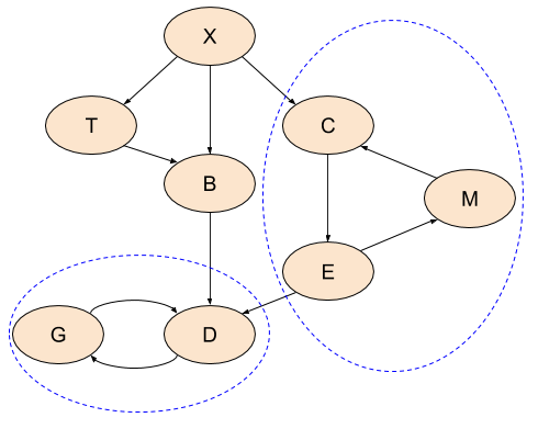
Having this decomposition of the graph availabe, we can now once again run meaningful post-order visits on the SCCs and even sort them topologically.
There are a number of efficient algorithms available for decomposing a graph into SCCs; I will leave this topic to some other time.
3-color DFS and edge classification
As we've seen above, while our postorder function manages to visit all nodes in a graph with cycles, it doesn't do it in a sensical order and doesn't even detect cycles. We'll now examine a variation of the DFS algorithm that keeps track of more information during traversal, which helps it analyze cyclic graphs with more insight.
This version of graph DFS is actually something you will often find in books and other references; it colors every node white, grey or black, depending on how much traversal was done from it at any given time. This is why I call it the "3-color" algorithm, as opposed to the basic "binary" or "2-color" algorithm presented here earlier (any node is either in the "visited" set or not).
The following function implements this. The color dict replaces the visited set and tracks three different states for each node:
- Node not in the dict: not discovered yet ("white").
- Node discovered but not finished yet ("grey")
- Node is finished - all its outgoing edges were finished ("black")
def postorder_3color(graph, root):
    """Return a post-order ordering of nodes in the graph.

    Prints CYCLE notifications when graph cycles ("back edges") are discovered.
    """
    color = dict()
    order = []
    def dfs_walk(node):
        color[node] = 'grey'
        for succ in graph.successors(node):
            if color.get(succ) == 'grey':
                print 'CYCLE: {0}-->{1}'.format(node, succ)
            if succ not in color:
                dfs_walk(succ)
        order.append(node)
        color[node] = 'black'
    dfs_walk(root)
    return order
If we run it on the loopy graph, we get the same order as the one returned by postorder, with the addition of:
CYCLE: m-->c
CYCLE: g-->d
The edges between M and C and between G and D are called back edges. This falls under the realm of edge classification. In addition to back edges, graphs can have tree edges, cross edges and forward edges. All of these can be discovered during a DFS visit. Back edges are the most important for our current discussion since they help us identify cycles in the graph.
Data-flow analysis
This section is optional if you only wanted to learn about graph graversals. It assumes non-trivial background on compilation.
In compilation, data-flow analysis is an important technique used for many optimizations. The compiler analyzes the control-flow graph (CFG) of a program, reasoning about how values can potentially change [6] through its basic blocks.
Without getting into the specifics of data-flow analysis problems and algorithms, I want to mention a few relevant observations that bear strong relation to the earlier topics of this post. Broadly speaking, there are two kinds of data-flow problems: forward and backward problems. In forward problems, we use information learned about basic blocks to analyze their successors. In backward problems, it's the other way around - information learned about basic blocks is used to analyze their predecessors.
Therefore, it shouldn't come as a surprise that the most efficient way to run forward data-flow analyses is in RPO. In the absence of cycles, RPO (topological order) makes sure we've seen all of a node's predecessors before we get to it. This means we can perform the analysis in a single pass over the graph.
With cycles in the graph, this is no longer true, but RPO still guarantees the fastest convergence - in graphs with cycles data-flow analysis is iterative until a fixed point is reached [7].
For a similar reason, the most efficient way to run backward data-flow analysis is post-order. In the absence of cycles, postorder makes sure that we've seen all of a node's successors before we get to it.
One final note: some resources recommend to use RPO on a reverse CFG (CFG with all its edges inverted) instead of post-order on the original graph for backward data-flow. If your initial reaction is to question whether the two are equivalent - that's not a bad guess, though it's wrong. With cycles, the two orders can be subtly different. Consider this graph, for example:
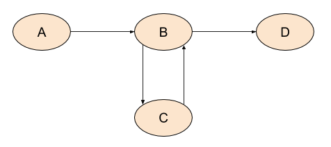
Assuming A is the entry node, post-order would return: D, C, B, A. Now let's invert all the edges:

Here D would be the entry node. RPO on this graph is: D, B, C, A. This is not the same as post-order on the original graph - the order of the nodes in the cycle is different.
So here's a puzzle: why is RPO on the reverse graph recommended by some resources over post-order?
If I had to guess, I'd say that looking at the sample graph in this section, it makes some sense to examine B before C, because more of its successors were already visited. If we visit C before B, we don't know much about successors yet because B wasn't visited - and B is the only successor of C. But if we visit B before C, at least D (a successor of B in the original graph) was already visited. This may help faster convergence. If you have additional ideas, please let me know.
| [1] | This depends on the order in which edges were added to the graph, the data structure this graph uses to store these edges, and the order the graph's successors methods returns node successors. The abstract algorithm doesn't enforce any of this. |
| [2] | There may be other reasons for V to come before W - for example if both are root nodes. |
| [3] | Its leftmost part has the same structure as our initial sample graph, with the slight difference of replacing A by X. I did this to shuffle the traversal order a bit; in my implementation, it happens to depend on the order Python's set.pop returns it elements. |
| [4] | It should be an easy exercise to figure out how the traversal got to return M first here. |
| [5] | This is only useful for fairly regular graphs, of course, If all nodes in a graph are reachable from one another (the whole graph is strongly connected), the SCC decomposition won't help much since the whole graph will be a single component. But then we also wouldn't have the problem of discovering M before G and D as in the sample graph. |
| [6] | I'm saying "potentially" because this is static analysis. In the general case, the compiler cannot know which conditions will be true and false at runtime - it can only use information available to it statically, before the program actually executes. |
| [7] | Since data-flow sets form a partial order and the algorithms have to satisfy some additional mathematical guarantees, it will converge even if we visit nodes randomly. However, picking the right order may result is significantly faster convergence - which is important for compiltation time. |